Data Science Fundamentals Pocket Primer E-Book

Mercury Learning and Information

• Herausgeber: Packt Publishing
• Kategorie: Lebensstil
• Sprache: Englisch

Seitenzahl: 590

Veröffentlichungsjahr: 2024

Beschreibung

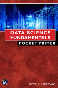
This book, part of the Pocket Primer series, introduces the basic concepts of data science using Python 3 and other applications. It offers a fast-paced introduction to data analytics, statistics, data visualization, linear algebra, and regular expressions. The book features numerous code samples using Python, NumPy, R, SQL, NoSQL, and Pandas. Companion files with source code and color figures are available.
Understanding data science is crucial in today's data-driven world. This book provides a comprehensive introduction, covering key areas such as Python 3, data visualization, and statistical concepts. The practical code samples and hands-on approach make it ideal for beginners and those looking to enhance their skills.
The journey begins with working with data, followed by an introduction to probability, statistics, and linear algebra. It then delves into Python, NumPy, Pandas, R, regular expressions, and SQL/NoSQL, concluding with data visualization techniques. This structured approach ensures a solid foundation in data science.

Leseprobe

DATA SCIENCEFUNDAMENTALS

Pocket Primer

LICENSE, DISCLAIMER OF LIABILITY, AND LIMITED WARRANTY

By purchasing or using this book and companion files (the “Work”), you agree that this license grants permission to use the contents contained herein, including the disc, but does not give you the right of ownership to any of the textual content in the book / disc or ownership to any of the information or products contained in it. This license does not permit uploading of the Work onto the Internet or on a network (of any kind) without the written consent of the Publisher. Duplication or dissemination of any text, code, simulations, images, etc. contained herein is limited to and subject to licensing terms for the respective products, and permission must be obtained from the Publisher or the owner of the content, etc., in order to reproduce or network any portion of the textual material (in any media) that is contained in the Work.

MERCURY LEARNINGAND INFORMATION (“MLI” or “the Publisher”) and anyone involved in the creation, writing, or production of the companion disc, accompanying algorithms, code, or computer programs (“the software”), and any accompanying Web site or software of the Work, cannot and do not warrant the performance or results that might be obtained by using the contents of the Work. The author, developers, and the Publisher have used their best efforts to ensure the accuracy and functionality of the textual material and/or programs contained in this package; we, however, make no warranty of any kind, express or implied, regarding the performance of these contents or programs. The Work is sold “as is” without warranty (except for defective materials used in manufacturing the book or due to faulty workmanship).

The author, developers, and the publisher of any accompanying content, and anyone involved in the composition, production, and manufacturing of this work will not be liable for damages of any kind arising out of the use of (or the inability to use) the algorithms, source code, computer programs, or textual material contained in this publication. This includes, but is not limited to, loss of revenue or profit, or other incidental, physical, or consequential damages arising out of the use of this Work.

The sole remedy in the event of a claim of any kind is expressly limited to replacement of the book and/or disc, and only at the discretion of the Publisher. The use of “implied warranty” and certain “exclusions” vary from state to state, and might not apply to the purchaser of this product.

Companion files for this title are available by writing to the publisher [email protected].

DATA SCIENCEFUNDAMENTALS

Pocket Primer

Oswald Campesato

Copyright ©2021 by MERCURY LEARNING AND INFORMATION LLC. All rights reserved.

This publication, portions of it, or any accompanying software may not be reproduced in any way, stored in a retrieval system of any type, or transmitted by any means, media, electronic display or mechanical display, including, but not limited to, photocopy, recording, Internet postings, or scanning, without prior permission in writing from the publisher.

Publisher: David Pallai

MERCURY LEARNINGAND INFORMATION

22841 Quicksilver Drive

Dulles, VA 20166

[email protected]

www.merclearning.com

800-232-0223

O. Campesato. Data Science Fundamentals Pocket Primer.

ISBN: 978-1-68392-733-4

The publisher recognizes and respects all marks used by companies, manufacturers, and developers as a means to distinguish their products. All brand names and product names mentioned in this book are trademarks or service marks of their respective companies. Any omission or misuse (of any kind) of service marks or trademarks, etc. is not an attempt to infringe on the property of others.

Library of Congress Control Number: 2021937777

212223321     This book is printed on acid-free paper in the United States of America.

Our titles are available for adoption, license, or bulk purchase by institutions, corporations, etc.For additional information, please contact the Customer Service Dept. at 800-232-0223(toll free).

All of our titles are available in digital format at academiccourseware.com and other digital vendors.Companion files (figures and code listings) for this title are available by contacting [email protected]. The sole obligation of MERCURY LEARNING AND INFORMATION to the purchaser is to replace the disc, based on defective materials or faulty workmanship, but not based on the operation or functionality of the product.

I’d like to dedicate this book to my parents-may this bring joy and happiness into their lives.

Contents

Preface

Chapter 1   Working With Data

What are Datasets?

Data Preprocessing

Data Types

Preparing Datasets

Discrete Data Versus Continuous Data

“Binning” Continuous Data

Scaling Numeric Data via Normalization

Scaling Numeric Data via Standardization

What to Look for in Categorical Data

Mapping Categorical Data to Numeric Values

Working with Dates

Working with Currency

Missing Data, Anomalies, and Outliers

Missing Data

Anomalies and Outliers

Outlier Detection

What is Data Drift?

What is Imbalanced Classification?

What is SMOTE?

SMOTE Extensions

Analyzing Classifiers (Optional)

What is LIME?

What is ANOVA?

The Bias-Variance Trade-Off

Types of Bias in Data

Summary

Chapter 2   Intro to Probability and Statistics

What is a Probability?

Calculating the Expected Value

Random Variables

Discrete versus Continuous Random Variables

Well-Known Probability Distributions

Fundamental Concepts in Statistics

The Mean

The Median

The Mode

The Variance and Standard Deviation

Population, Sample, and Population Variance

Chebyshev’s Inequality

What is a P-Value?

The Moments of a Function (Optional)

What is Skewness?

What is Kurtosis?

Data and Statistics

The Central Limit Theorem

Correlation versus Causation

Statistical Inferences

Statistical Terms – RSS, TSS, R^2, and F1 Score

What is an F1 Score?

Gini Impurity, Entropy, and Perplexity

What is the Gini Impurity?

What is Entropy?

Calculating Gini Impurity and Entropy Values

Multidimensional Gini Index

What is Perplexity?

Cross-Entropy and KL Divergence

What is Cross-Entropy?

What is KL Divergence?

What’s their Purpose?

Covariance and Correlation Matrices

The Covariance Matrix

Covariance Matrix: An Example

The Correlation Matrix

Eigenvalues and Eigenvectors

Calculating Eigenvectors: A Simple Example

Gauss Jordan Elimination (Optional)

PCA (Principal Component Analysis)

The New Matrix of Eigenvectors

Well-Known Distance Metrics

Pearson Correlation Coefficient

Jaccard Index (or Similarity)

Local Sensitivity Hashing (Optional)

Types of Distance Metrics

What is Bayesian Inference?

Bayes’ Theorem

Some Bayesian Terminology

What is MAP?

Why Use Bayes’ Theorem?

Summary

Chapter 3   Linear Algebra Concepts

What is Linear Algebra?

What are Vectors?

The Norm of a Vector

The Inner Product of Two Vectors

The Cosine Similarity of Two Vectors

Bases and Spanning Sets

Three Dimensional Vectors and Beyond

What are Matrices?

Add and Multiply Matrices

The Determinant of a Square Matrix

Well-Known Matrices

Properties of Orthogonal Matrices

Operations Involving Vectors and Matrices

Gauss Jordan Elimination (Optional)

Covariance and Correlation Matrices

The Covariance Matrix

Covariance Matrix: An Example

The Correlation Matrix

Eigenvalues and Eigenvectors

Calculating Eigenvectors: A Simple Example

What is PCA (Principal Component Analysis)?

The Main Steps in PCA

The New Matrix of Eigenvectors

Dimensionality Reduction

Dimensionality Reduction Techniques

The Curse of Dimensionality

SVD (Singular Value Decomposition)

LLE (Locally Linear Embedding)

UMAP

t-SNE

PHATE

Linear Versus Non-Linear Reduction Techniques

Complex Numbers (Optional)

Complex Numbers on the Unit Circle

Complex Conjugate Root Theorem

Hermitian Matrices

Summary

Chapter 4   Introduction to Python

Tools for Python

easy_install and pip

virtualenv

Python Installation

Setting the PATH Environment Variable (Windows Only)

Launching Python on Your Machine

The Python Interactive Interpreter

Python Identifiers

Lines, Indentations, and Multi-Lines

Quotation and Comments in Python

Saving Your Code in a Module

Some Standard Modules in Python

The help() and dir() Functions

Compile Time and Runtime Code Checking

Simple Data Types in Python

Working with Numbers

Working with Other Bases

The chr() Function

The round() Function in Python

Formatting Numbers in Python

Unicode and UTF-8

Working with Unicode

Working with Strings

Comparing Strings

Formatting Strings in Python

Uninitialized Variables and the Value None in Python

Slicing and Splicing Strings

Testing for Digits and Alphabetic Characters

Search and Replace a String in Other Strings

Remove Leading and Trailing Characters

Printing Text without NewLine Characters

Text Alignment

Working with Dates

Converting Strings to Dates

Exception Handling in Python

Handling User Input

Command-Line Arguments

Precedence of Operators in Python

Python Reserved Words

Working with Loops in Python

Python For Loops

A For Loop with try/except in Python

Numeric Exponents in Python

Nested Loops

The split() Function with For Loops

Using the split() Function to Compare Words

Using the split() Function to Print Justified Text

Using the split() Function to Print Fixed Width Text

Using the split() Function to Compare Text Strings

Using the split() Function to Display Characters in a String

The join() Function

Python While Loops

Conditional Logic in Python

The break/continue/pass Statements

Comparison and Boolean Operators

The in/not in/is/is not Comparison Operators

The and, or, and not Boolean Operators

Local and Global Variables

Scope of Variables

Pass by Reference Versus Value

Arguments and Parameters

Using a While Loop to Find the Divisors of a Number

Using a While Loop to Find Prime Numbers

User-Defined Functions in Python

Specifying Default Values in a Function

Returning Multiple Values from a Function

Functions with a Variable Number of Arguments

Lambda Expressions

Recursion

Calculating Factorial Values

Calculating Fibonacci Numbers

Working with Lists

Lists and Basic Operations

Reversing and Sorting a List

Lists and Arithmetic Operations

Lists and Filter-related Operations

Sorting Lists of Numbers and Strings

Expressions in Lists

Concatenating a List of Words

The Python range() Function

Counting Digits, Uppercase, and Lowercase Letters

Arrays and the append() Function

Working with Lists and the split() Function

Counting Words in a List

Iterating Through Pairs of Lists

Other List-Related Functions

Working with Vectors

Working with Matrices

Queues

Tuples (Immutable Lists)

Sets

Dictionaries

Creating a Dictionary

Displaying the Contents of a Dictionary

Checking for Keys in a Dictionary

Deleting Keys from a Dictionary

Iterating Through a Dictionary

Interpolating Data from a Dictionary

Dictionary Functions and Methods

Dictionary Formatting

Ordered Dictionaries

Sorting Dictionaries

Python Multi Dictionaries

Other Sequence Types in Python

Mutable and Immutable Types in Python

The type() Function

Summary

Chapter 5   Introduction to NumPy

What is NumPy?

Useful NumPy Features

What are NumPy Arrays?

Working with Loops

Appending Elements to Arrays (1)

Appending Elements to Arrays (2)

Multiplying Lists and Arrays

Doubling the Elements in a List

Lists and Exponents

Arrays and Exponents

Math Operations and Arrays

Working with “-1” Sub-ranges with Vectors

Working with “-1” Sub-ranges with Arrays

Other Useful NumPy Methods

Arrays and Vector Operations

NumPy and Dot Products (1)

NumPy and Dot Products (2)

NumPy and the Length of Vectors

NumPy and Other Operations

NumPy and the reshape() Method

Calculating the Mean and Standard Deviation

Code Sample with Mean and Standard Deviation

Trimmed Mean and Weighted Mean

Working with Lines in the Plane (Optional)

Plotting Randomized Points with NumPy and Matplotlib

Plotting a Quadratic with NumPy and Matplotlib

What is Linear Regression?

What is Multivariate Analysis?

What about Non-Linear Datasets?

The MSE (Mean Squared Error) Formula

Other Error Types

Non-Linear Least Squares

Calculating the MSE Manually

Find the Best-Fitting Line in NumPy

Calculating MSE by Successive Approximation (1)

Calculating MSE by Successive Approximation (2)

Google Colaboratory

Uploading CSV Files in Google Colaboratory

Summary

Chapter 6   Introduction to Pandas

What is Pandas?

Pandas Options and Settings

Pandas Data Frames

Data Frames and Data Cleaning Tasks

Alternatives to Pandas

A Pandas Data Frame with a NumPy Example

Describing a Pandas Data Frame

Pandas Boolean Data Frames

Transposing a Pandas Data Frame

Pandas Data Frames and Random Numbers

Reading CSV Files in Pandas

The loc() and iloc() Methods in Pandas

Converting Categorical Data to Numeric Data

Matching and Splitting Strings in Pandas

Converting Strings to Dates in Pandas

Merging and Splitting Columns in Pandas

Combining Pandas Data Frames

Data Manipulation with Pandas Data Frames (1)

Data Manipulation with Pandas Data Frames (2)

Data Manipulation with Pandas Data Frames (3)

Pandas Data Frames and CSV Files

Managing Columns in Data Frames

Switching Columns

Appending Columns

Deleting Columns

Inserting Columns

Scaling Numeric Columns

Managing Rows in Pandas

Selecting a Range of Rows in Pandas

Finding Duplicate Rows in Pandas

Inserting New Rows in Pandas

Handling Missing Data in Pandas

Multiple Types of Missing Values

Test for Numeric Values in a Column

Replacing NaN Values in Pandas

Sorting Data Frames in Pandas

Working with groupby() in Pandas

Working with apply() and mapapply() in Pandas

Handling Outliers in Pandas

Pandas Data Frames and Scatterplots

Pandas Data Frames and Simple Statistics

Aggregate Operations in Pandas Data Frames

Aggregate Operations with the titanic.csv Dataset

Save Data Frames as CSV Files and Zip Files

Pandas Data Frames and Excel Spreadsheets

Working with JSON-based Data

Python Dictionary and JSON

Python, Pandas, and JSON

Useful One-line Commands in Pandas

What is Method Chaining?

Pandas and Method Chaining

Pandas Profiling

Summary

Chapter 7   Introduction to R

What is R?

Features of R

Installing R and RStudio

Variable Names, Operators, and Data Types in R

Assigning Values to Variables in R

Operators in R

Data Types in R

Working with Strings in R

Uppercase and Lowercase Strings

String-Related Tasks

Working with Vectors in R

Finding NULL Values in a Vector in R

Updating NA Values in a Vector in R

Sorting a Vector of Elements in R

Working with the Alphabet Variable in R

Working with Lists in R

Working with Matrices in R (1)

Working with Matrices in R (2)

Working with Matrices in R (3)

Working with Matrices in R (4)

Working with Matrices in R (5)

Updating Matrix Elements

Logical Constraints and Matrices

Working with Matrices in R (6)

Combining Vectors, Matrices, and Lists in R

Working with Dates in R

The seq Function in R

Basic Conditional Logic

Compound Conditional Logic

Working with User Input

A Try/Catch Block in R

Linear Regression in R

Working with Simple Loops in R

Working with Nested Loops in R

Working with While Loops in R

Working with Conditional Logic in R

Add a Sequence of Numbers in R

Check if a Number is Prime in R

Check if Numbers in an Array are Prime in R

Check for Leap Years in R

Well-formed Triangle Values in R

What are Factors in R?

What are Data Frames in R?

Working with Data Frames in R (1)

Working with Data Frames in R (2)

Working with Data frames in R (3)

Sort a Data Frame by Column

Reading Excel Files in R

Reading SQLITE Tables in R

Reading Text Files in R

Saving and Restoring Objects in R

Data Visualization in R

Working with Bar Charts in R (1)

Working with Bar Charts in R (2)

Working with Line Graphs in R

Working with Functions in R

Math-related Functions in R

Some Operators and Set Functions in R

The “Apply Family” of Built-in Functions

The dplyr Package in R

The Pipe Operator %>%

Working with CSV Files in R

Working with XML in R

Reading an XML Document into an R Data Frame

Working with JSON in R

Reading a JSON File into an R Data Frame

Statistical Functions in R

Summary Functions in R

Defining a Custom Function in R

Recursion in R

Calculating Factorial Values in R (Non-recursive)

Calculating Factorial Values in R (recursive)

Calculating Fibonacci Numbers in R (Non-recursive)

Calculating Fibonacci Numbers in R (Recursive)

Convert a Decimal Integer to a Binary Integer in R

Calculating the GCD of Two Integers in R

Calculating the LCM of Two Integers in R

Summary

Chapter 8   Regular Expressions

What are Regular Expressions?

Metacharacters in Python

Character Sets in Python

Working with “^” and “\”

Character Classes in Python

Matching Character Classes with the re Module

Using the re.match() Method

Options for the re.match() Method

Matching Character Classes with the re.search() Method

Matching Character Classes with the findAll() Method

Finding Capitalized Words in a String

Additional Matching Function for Regular Expressions

Grouping with Character Classes in Regular Expressions

Using Character Classes in Regular Expressions

Matching Strings with Multiple Consecutive Digits

Reversing Words in Strings

Modifying Text Strings with the re Module

Splitting Text Strings with the re.split() Method

Splitting Text Strings Using Digits and Delimiters

Substituting Text Strings with the re.sub() Method

Matching the Beginning and the End of Text Strings

Compilation Flags

Compound Regular Expressions

Counting Character Types in a String

Regular Expressions and Grouping

Simple String Matches

Pandas and Regular Expressions

Summary

Exercises

Chapter 9   SQL and NoSQL

What is an RDBMS?

A Four-Table RDBMS

The customers Table

The purchase_orders Table

The line_items Table

The item_desc Table

What is SQL?

What is DCL?

What is DDL?

Delete Vs. Drop Vs. Truncate

What is DQL?

What is DML?

What is TCL?

Data Types in MySQL

Working with MySQL

Logging into MySQL

Creating a MySQL Database

Creating and Dropping Tables

Manually Creating Tables for mytools.com

Creating Tables via a SQL Script for mytools.com (1)

Creating Tables via a SQL Script for mytools.com (2)

Creating Tables from the Command Line

Dropping Tables via a SQL Script for mytools.com

Populating Tables with Seed Data

Populating Tables from Text Files

Simple SELECT Statements

Select Statements with a WHERE Clause

Select Statements with GROUP BY Clause

Select Statements with a HAVING Clause

Working with Indexes in SQL

What are Keys in an RDBMS?

Aggregate and Boolean Operations in SQL

Joining Tables in SQL

Defining Views in MySQL

Entity Relationships

One-to-Many Entity Relationships

Many-to-Many Entity Relationships

Self-Referential Entity Relationships

Working with Subqueries in SQL

Other Tasks in SQL

Reading MySQL Data from Pandas

Export SQL Data to Excel

What is Normalization?

What are Schemas?

Other RDBMS Topics

Working with NoSQL

Create MongoDB Cellphones Collection

Sample Queries in MongoDB

Summary

Chapter 10   Data Visualization

What is Data Visualization?

Types of Data Visualization

What is Matplotlib?

Horizontal Lines in Matplotlib

Slanted Lines in Matplotlib

Parallel Slanted Lines in Matplotlib

A Grid of Points in Matplotlib

A Dotted Grid in Matplotlib

Lines in a Grid in Matplotlib

A Colored Grid in Matplotlib

A Colored Square in an Unlabeled Grid in Matplotlib

Randomized Data Points in Matplotlib

A Histogram in Matplotlib

A Set of Line Segments in Matplotlib

Plotting Multiple Lines in Matplotlib

Trigonometric Functions in Matplotlib

Display IQ Scores in Matplotlib

Plot a Best-Fitting Line in Matplotlib

Introduction to Sklearn (scikit-learn)

The Digits Dataset in Sklearn

The Iris Dataset in Sklearn (1)

Sklearn, Pandas, and the Iris Dataset

The Iris Dataset in Sklearn (2)

The Faces Dataset in Sklearn (Optional)

Working with Seaborn

Features of Seaborn

Seaborn Built-in Datasets

The Iris Dataset in Seaborn

The Titanic Dataset in Seaborn

Extracting Data from the Titanic Dataset in Seaborn (1)

Extracting Data from the Titanic Dataset in Seaborn (2)

Visualizing a Pandas Dataset in Seaborn

Data Visualization in Pandas

What is Bokeh?

Summary

Index

Preface

WHAT IS THE PRIMARY VALUE PROPOSITION FOR THIS BOOK?

This book contains a fast-paced introduction to as much relevant information about data analytics as possible that can be reasonably included in a book of this size. Please keep in mind the following point: this book is intended to provide you with a broad overview of many relevant technologies.

As such, you will be exposed to a variety of features of NumPy and Pandas, how to write regular expressions (with an accompanying chapter), and how to perform many data cleaning tasks. Keep in mind that some topics are presented in a cursory manner, which is for two main reasons. First, it’s important that you be exposed to these concepts. In some cases, you will find topics that might pique your interest, and hence motivate you to learn more about them through self-study; in other cases, you will probably be satisfied with a brief introduction. In other words, you can decide whether to delve into more detail regarding the topics in this book.

Second, a full treatment of all the topics that are covered in this book would significantly increase the size of this book.

However, it’s important for you to decide if this approach is suitable for your needs and learning style. If not, you can select one or more of the plethora of data analytics books that are available.

THE TARGET AUDIENCE

This book is intended primarily for people who have worked with Python and are interested in learning about several important Python libraries, such as NumPy and Pandas.

This book is also intended to reach an international audience of readers with highly diverse backgrounds. While many readers know how to read English, their native spoken language is not English. Consequently, this book uses standard English rather than colloquial expressions that might be confusing to those readers. As you know, many people learn by different types of imitation, which includes reading, writing, or hearing new material. This book takes these points into consideration to provide a comfortable and meaningful learning experience for the intended readers.

WHAT WILL I LEARN FROM THIS BOOK?

The first chapter contains a quick tour of basic Python 3, followed by a chapter that introduces you to data types and data cleaning tasks, such as working with datasets that contain different types of data and how to handle missing data. The third and fourth chapters introduce you to NumPy and Pandas (and many code samples).

The fifth chapter contains fundamental concepts in probability and statistics, such as mean, mode, and variance and correlation matrices. You will also learn about Gini impurity, entropy, and KL-divergence. You will also learn about eigenvalues, eigenvectors, and PCA (Principal Component Analysis).

The sixth chapter of this book delves into Pandas, followed by Chapter 7 about R programming. Chapter 8 covers regular expressions and provides with plenty of examples. Chapter 9 discusses both SQL and NoSQL, and then Chapter 10 discusses data visualization with numerous code samples for Matplotlib, Seaborn, and Bokeh.

WHY ARE THE CODE SAMPLES PRIMARILY IN PYTHON?

Most of the code samples are short (usually less than one page and sometimes less than half a page), and if need be, you can easily and quickly copy/paste the code into a new Jupyter notebook. For the Python code samples that reference a CSV file, you do not need any additional code in the corresponding Jupyter notebook to access the CSV file. Moreover, the code samples execute quickly, so you won’t need to avail yourself of the free GPU that is provided in Google Colaboratory.

If you do decide to use Google Colaboratory, you can avail yourself of many useful features of Colaboratory (e.g., the upload feature to upload existing Jupyter notebooks). If the Python code references a CSV file, make sure that you include the appropriate code snippet (as explained in Chapter 1) to access the CSV file in the corresponding Jupyter notebook in Google Colaboratory.

DO I NEED TO LEARN THE THEORY PORTIONS OF THIS BOOK?

Once again, the answer depends on the extent to which you plan to become involved in data analytics. For example, if you plan to study machine learning, then you will probably learn how to create and train a model, which is a task that is performed after data cleaning tasks. In general, you will probably need to learn everything that you encounter in this book if you are planning to become a machine learning engineer.

WHY DOES THIS BOOK INCLUDE SKLEARN MATERIAL?

The Sklearn material in this book is minimalistic because this book is not about machine learning. The Sklearn material is located in Chapter 6, where you will learn about some of the Sklearn built-in datasets. If you decide to delve into machine learning, you will have already been introduced to some aspects of Sklearn.

WHY IS A REGEX CHAPTER INCLUDED IN THIS BOOK?

Regular expressions are supported in multiple languages (including Java and JavaScript) and they enable you to perform complex tasks with very compact regular expressions. Regular expressions can seem arcane and too complex to learn in a reasonable amount of time. Chapter 2 contains some Pandas-based code samples that use regular expressions to perform tasks that might otherwise be more complicated.

If you plan to use Pandas extensively or you plan to work on NLP-related tasks, then the code samples in this chapter will be very useful for you because they are more than adequate for solving certain types of tasks, such as removing HTML tags. Moreover, your knowledge of RegEx will transfer instantly to other languages that support regular expressions.

GETTING THE MOST FROM THIS BOOK

Some programmers learn well from prose, others learn well from sample code (and lots of it), which means that there’s no single style that can be used for everyone.

Moreover, some programmers want to run the code first, see what it does, and then return to the code to delve into the details (and others use the opposite approach).

Consequently, there are various types of code samples in this book: some are short, some are long, and other code samples “build” from earlier code samples.

WHAT DO I NEED TO KNOW FOR THIS BOOK?

Current knowledge of Python 3.x is the most helpful skill. Knowledge of other programming languages (such as Java) can also be helpful because of the exposure to programming concepts and constructs. The less technical knowledge that you have, the more diligence will be required to understand the various topics that are covered.

If you want to be sure that you can grasp the material in this book, glance through some of the code samples to get an idea of how much is familiar to you and how much is new for you.

DOESN’T THE COMPANION FILES OBVIATE THE NEED FOR THIS BOOK?

The companion files contains all the code samples to save you time and effort from the error-prone process of manually typing code into a text file. In addition, there are situations in which you might not have easy access to the companion files. Furthermore, the code samples in the book provide explanations that are not available on the companion files.

DOES THIS BOOK CONTAIN PRODUCTION-LEVEL CODE SAMPLES?

The primary purpose of the code samples in this book is to show you Python-based libraries for solving a variety of data-related tasks in conjunction with acquiring a rudimentary understanding of statistical concepts. Clarity has higher priority than writing more compact code that is more difficult to understand (and possibly more prone to bugs). If you decide to use any of the code in this book in a production website, you should subject that code to the same rigorous analysis as the other parts of your code base.

WHAT ARE THE NON-TECHNICAL PREREQUISITES FOR THIS BOOK?

Although the answer to this question is more difficult to quantify, it’s important to have strong desire to learn about data science, along with the motivation and discipline to read and understand the code samples.

HOW DO I SET UP A COMMAND SHELL?

If you are a Mac user, there are three ways to do so. The first method is to use Finder to navigate to Applications > Utilities and then double click on the Utilities application. Next, if you already have a command shell available, you can launch a new command shell by typing the following command:

open /Applications/Utilities/Terminal.app

A second method for Mac users is to open a new command shell on a Macbook from a command shell that is already visible simply by clicking command+n in that command shell, and your Mac will launch another command shell.

If you are a PC user, you can install Cygwin (which is open source: https://cygwin.com/) that simulates bash commands, or use another toolkit such as MKS (a commercial product). Please read the online documentation that describes the download and installation process. Note that custom aliases are not automatically set if they are defined in a file other than the main start-up file (such as .bash_login).

COMPANION FILES

All the code samples and figures in this book may be obtained by writing to the publisher at [email protected].

WHAT ARE THE NEXT STEPS AFTER FINISHING THIS BOOK?

The answer to this question varies widely, mainly because the answer depends heavily on your objectives. If you are interested primarily in NLP, then you can learn more advanced concepts, such as attention, transformers, and the BERT-related models.

If you are primarily interested in machine learning, there are some subfields of machine learning, such as deep learning and reinforcement learning (and deep reinforcement learning) that might appeal to you. Fortunately, there are many resources available, and you can perform an Internet search for those resources. One other point: the aspects of machine learning for you to learn depend on who you are. The needs of a machine learning engineer, data scientist, manager, student, or software developer are all different.

Oswald CampesatoApril 2021

CHAPTER 1

WORKING WITH DATA

This chapter introduces you to data types, how to scale data values, and various techniques for handling missing data values. If most of the material in this chapter is new to you, be assured that it’s not necessary to understand everything in this chapter. It’s still a good idea to read as much material as you can absorb, and perhaps return to this chapter again after you have completed some of the other chapters in this book.

The first part of this chapter contains an overview of different types of data and an explanation of how to normalize and standardize a set of numeric values by calculating the mean and standard deviation of a set of numbers. You will see how to map categorical data to a set of integers and how to perform one-hot encoding.

The second part of this chapter discusses missing data, outliers, and anomalies, as well as some techniques for handling these scenarios. The third section discusses imbalanced data and the use of SMOTE (Synthetic Minority Oversampling Technique) to deal with imbalanced classes in a dataset.

The fourth section discusses ways to evaluate classifiers such as LIME and ANOVA. This section also contains details regarding the bias-variance trade-off and various types of statistical bias.

WHAT ARE DATASETS?

In simple terms, a dataset is a source of data (such as a text file) that contains rows and columns of data. Each row is typically called a data point, and each column is called a feature. A dataset can be in a range of formats: CSV (comma separated values), TSV (tab separated values), Excel spreadsheet, a table in an RDMBS (Relational Database Management Systems), a document in a NoSQL database, or the output from a Web service. Someone needs to analyze the dataset to determine which features are the most important and which features can be safely ignored to train a model with the given dataset.

A dataset can vary from very small (a couple of features and 100 rows) to very large (more than 1,000 features and more than one million rows). If you are unfamiliar with the problem domain, then you might struggle to determine the most important features in a large dataset. In this situation, you might need a domain expert who understands the importance of the features, their interdependencies (if any), and whether the data values for the features are valid. In addition, there are algorithms (called dimensionality reduction algorithms) that can help you determine the most important features. For example, PCA (Principal Component Analysis) is one such algorithm, which is discussed in more detail in Chapter 2.

Data Preprocessing

Data preprocessing is the initial step that involves validating the contents of a dataset, which involves making decisions about missing data, duplicate data, and incorrect data values:

dealing with missing data values

cleaning “noisy” text-based data

removing HTML tags

removing emoticons

dealing with emojis/emoticons

filtering data

grouping data

handling currency and date formats (i18n)

Cleaning data is done before data wrangling that involves removing unwanted data as well as handling missing data. In the case of text-based data, you might need to remove HTML tags and punctuation. In the case of numeric data, it’s less likely (though still possible) that alphabetic characters are mixed together with numeric data. However, a dataset with numeric features might have incorrect values or missing values (discussed later). In addition, calculating the minimum, maximum, mean, median, and standard deviation of the values of a feature obviously pertain only to numeric values.

After the preprocessing step is completed, data wrangling is performed, which refers to transforming data into a new format. You might have to combine data from multiple sources into a single dataset. For example, you might need to convert between different units of measurement (such as date formats or currency values) so that the data values can be represented in a consistent manner in a dataset.

Currency and date values are part of i18n (internationalization), whereas l10n (localization) targets a specific nationality, language, or region. Hard-coded values (such as text strings) can be stored as resource strings in a file called a resource bundle, where each string is referenced via a code. Each language has its own resource bundle.

DATA TYPES

Explicit data types exist in many programming languages, such as C, C++, Java, and TypeScript. Some programming languages, such as JavaScript and awk, do not require initializing variables with an explicit type: the type of a variable is inferred dynamically via an implicit type system (i.e., one that is not directly exposed to a developer).

In machine learning, datasets can contain features that have different types of data, such as a combination of one or more of the following:

numeric data (integer/floating point and discrete/continuous)

character/categorical data (different languages)

date-related data (different formats)

currency data (different formats)

binary data (yes/no, 0/1, and so forth)

nominal data (multiple unrelated values)

ordinal data (multiple and related values)

Consider a dataset that contains real estate data, which can have as many as thirty columns (or even more), often with the following features:

the number of bedrooms in a house: numeric value and a discrete value

the number of square feet: a numeric value and (probably) a continuous value

the name of the city: character data

the construction date: a date value

the selling price: a currency value and probably a continuous value

the “for sale” status: binary data (either “yes” or “no”)

An example of nominal data is the seasons in a year. Although many (most?) countries have four distinct seasons, some countries have two distinct seasons. However, keep in mind that seasons can be associated with different temperature ranges (summer versus winter). An example of ordinal data is an employee’s pay grade: 1=entry level, 2=one year of experience, and so forth. Another example of nominal data is a set of colors, such as {Red, Green, Blue}.

An example of binary data is the pair {Male, Female}, and some datasets contain a feature with these two values. If such a feature is required for training a model, first convert {Male, Female} to a numeric counterpart, such as {0,1}. Similarly, if you need to include a feature whose values are the previous set of colors, you can replace {Red, Green, Blue} with the values {0,1,2}. Categorical data is discussed in more detail later in this chapter.

MISSING DATA, ANOMALIES, AND OUTLIERS

Although missing data is not directly related to checking for anomalies and outliers, in general you will perform all three of these tasks. Each task involves a set of techniques to help you perform an analysis of the data in a dataset, and the following subsections describe some of those techniques.

Missing Data

How you decide to handle missing data depends on the specific dataset. Here are some ways to handle missing data (the first three techniques are manual techniques, and the other techniques are algorithms):

Replace missing data with the mean/median/mode value.

Infer (“impute”) the value for missing data.

Delete rows with missing data.

Isolation forest (tree-based algorithm).

Use the minimum covariance determinant.

Use the local outlier factor.

Use the one-class SVM (Support Vector Machines).

In general, replacing a missing numeric value with zero is a risky choice: this value is obviously incorrect if the values of a feature are between 1,000 and 5,000. For a feature that has numeric values, replacing a missing value with the average value is better than the value zero (unless the average equals zero); also consider using the median value. For categorical data, consider using the mode to replace a missing value.

If you are not confident that you can impute a “reasonable” value, consider excluding the row with a missing value, and then train a model with the imputed value and the deleted row.

One problem that can arise after removing rows with missing values is that the resulting dataset is too small. In this case, consider using SMOTE, which is discussed later in this chapter, to generate synthetic data.

Anomalies and Outliers

In simplified terms, an outlier is an abnormal data value that is outside the range of “normal” values. For example, a person’s height in centimeters is typically between 30 centimeters and 250 centimeters. Hence, a data point (e.g., a row of data in a spreadsheet) with a height of 5 centimeters or a height of 500 centimeters is an outlier. The consequences of these outlier values are unlikely to involve a significant financial or physical loss (though they could adversely affect the accuracy of a trained model).

Anomalies are also outside the “normal” range of values (just like outliers), and they are typically more problematic than outliers: anomalies can have more severe consequences than outliers. For example, consider the scenario in which someone who lives in California suddenly makes a credit card purchase in New York. If the person is on vacation (or a business trip), then the purchase is an outlier (it’s outside the typical purchasing pattern), but it’s not an issue. However, if that person was in California when the credit card purchase was made, then it’s more likely to be credit card fraud, as well as an anomaly.

Unfortunately, there is no simple way to decide how to deal with anomalies and outliers in a dataset. Although you can exclude rows that contain outliers, keep in mind that doing so might deprive the dataset—and therefore the trained model—of valuable information. You can try modifying the data values (described as follows), but again, this might lead to erroneous inferences in the trained model. Another possibility is to train a model with the dataset that contains anomalies and outliers, and then train a model with a dataset from which the anomalies and outliers have been removed. Compare the two results and see if you can infer anything meaningful regarding the anomalies and outliers.

Outlier Detection

Although the decision to keep or drop outliers is your decision to make, there are some techniques available that help you detect outliers in a dataset. This section contains a short list of some techniques, along with a very brief description and links for additional information.

Perhaps trimming is the simplest technique (apart from dropping outliers), which involves removing rows whose feature value is in the upper 5% range or the lower 5% range. Winsorizing the data is an improvement over trimming. Set the values in the top 5% range equal to the maximum value in the 95th percentile, and set the values in the bottom 5% range equal to the minimum in the 5th percentile.

The Minimum Covariance Determinant is a covariance-based technique, and a Python-based code sample that uses this technique can be found online:

https://scikit-learn.org/stable/modules/outlier_detection.html.

The Local Outlier Factor (LOF) technique is an unsupervised technique that calculates a local anomaly score via the kNN (k Nearest Neighbor) algorithm. Documentation and short code samples that use LOF can be found online:

https://scikit-learn.org/stable/modules/generated/sklearn.neighbors.LocalOutlierFactor.html.

Two other techniques involve the Huber and the Ridge classes, both of which are included as part of Sklearn. The Huber error is less sensitive to outliers because it’s calculated via linear loss, similar to MAE (Mean Absolute Error). A code sample that compares Huber and Ridge can be found online:

https://scikit-learn.org/stable/auto_examples/linear_model/plot_huber_vs_ridge.html.

You can also explore the Theil-Sen estimator and RANSAC, which are “robust” against outliers, and additional information can be found online:

https://scikit-learn.org/stable/auto_examples/linear_model/plot_theilsen.html and https://en.wikipedia.org/wiki/Random_sample_consensus.

Four algorithms for outlier detection are discussed at the following site:

https://www.kdnuggets.com/2018/12/four-techniques-outlier-detection.html.

One other scenario involves “local” outliers. For example, suppose that you use kMeans (or some other clustering algorithm) and determine that a value is an outlier with respect to one of the clusters. While this value is not necessarily an “absolute” outlier, detecting such a value might be important for your use case.

What Is Data Drift?

The value of data is based on its accuracy, its relevance, and its age. Data drift refers to data that has become less relevant over time. For example, online purchasing patterns in 2010 are probably not as relevant as data from 2020 because of various factors (such as the profile of different types of customers). Keep in mind that there might be multiple factors that can influence data drift in a specific dataset.

Two techniques are domain classifier and the black-box shift detector, both of which can be found online:

https://blog.dataiku.com/towards-reliable-mlops-with-drift-detectors.

WHAT IS IMBALANCED CLASSIFICATION?

Imbalanced classification involves datasets with imbalanced classes. For example, suppose that class A has 99% of the data and class B has 1%. Which classification algorithm would you use? Unfortunately, classification algorithms don’t work well with this type of imbalanced dataset. Here is a list of several well-known techniques for handling imbalanced datasets:

Random resampling rebalances the class distribution.

Random oversampling duplicates data in the minority class.

Random undersampling deletes examples from the majority class.

SMOTE

Random resampling transforms the training dataset into a new dataset, which is effective for imbalanced classification problems.

The random undersampling technique removes samples from the dataset, and involves the following:

randomly remove samples from the majority class

can be performed with or without replacement

alleviates imbalance in the dataset

may increase the variance of the classifier

may discard useful or important samples

However, random undersampling does not work so well with a dataset that has a 99%/1% split into two classes. Moreover, undersampling can result in losing information that is useful for a model.

Instead of random undersampling, another approach involves generating new samples from a minority class. The first technique involves oversampling examples in the minority class and duplicate examples from the minority class.

There is another technique that is better than the preceding technique, which involves the following:

synthesizing new examples from a minority class

a type of data augmentation for tabular data

generating new samples from a minority class

Another well-known technique is called SMOTE, which involves data augmentation (i.e., synthesizing new data samples) well before you use a classification algorithm. SMOTE was initially developed by means of the kNN algorithm (other options are available), and it can be an effective technique for handling imbalanced classes.

Yet another option to consider is the Python package imbalanced-learn in the scikit-learn-contrib project. This project provides various re-sampling techniques for datasets that exhibit class imbalance. More details are available online:

https://github.com/scikit-learn-contrib/imbalanced-learn.

WHAT IS SMOTE?

SMOTE is a technique for synthesizing new samples for a dataset. This technique is based on linear interpolation:

Step 1: Select samples that are close in the feature space.

Step 2: Draw a line between the samples in the feature space.

Step 3: Draw a new sample at a point along that line.

A more detailed explanation of the SMOTE algorithm is here:

Select a random sample “a” from the minority class.

Now find k nearest neighbors for that example.

Select a random neighbor “b” from the nearest neighbors.

Create a line L that connects “a” and “b.”

Randomly select one or more points “c” on line L.

If need be, you can repeat this process for the other (k-1) nearest neighbors to distribute the synthetic values more evenly among the nearest neighbors.

SMOTE Extensions

The initial SMOTE algorithm is based on the kNN classification algorithm, which has been extended in various ways, such as replacing kNN with SVM. A list of SMOTE extensions is shown as follows:

selective synthetic sample generation

Borderline-SMOTE (kNN)

Borderline-SMOTE (SVM)

Adaptive Synthetic Sampling (ADASYN)

More information can be found online:

https://en.wikipedia.org/wiki/Oversampling_and_undersampling_in_data_analysis.

ANALYZING CLASSIFIERS (OPTIONAL)

This section is marked optional because its contents pertain to machine learning classifiers, which are not the focus of this book. However, it’s still worthwhile to glance through the material, or perhaps return to this section after you have a basic understanding of machine learning classifiers.

Several well-known techniques are available for analyzing the quality of machine learning classifiers. Two techniques are LIME and ANOVA, both of which are discussed in the following subsections.

What is LIME?

LIME is an acronym for Local Interpretable Model-Agnostic Explanations. LIME is a model-agnostic technique that can be used with machine learning models. The methodology of this technique is straightforward: make small random changes to data samples and then observe the manner in which predictions change (or not). The approach involves changing the data just a little and then observing what happens to the output.

By way of contrast, consider food inspectors who test for bacteria in truckloads of perishable food. Clearly, it’s infeasible to test every food item in a truck (or a train car), so inspectors perform “spot checks” that involve testing randomly selected items. Instead of sampling data, LIME makes small changes to input data in random locations and then analyzes the changes in the associated output values.

However, there are two caveats to keep in mind when you use LIME with input data for a given model:

The actual changes to input values are model-specific.

This technique works on input that is interpretable.