Introduction To Financial Modelling E-Book

MrExcel's Holy Macro! Books

• Herausgeber: Packt Publishing
• Kategorie: Lebensstil
• Sprache: Englisch

Seitenzahl: 390

Veröffentlichungsjahr: 2024

Beschreibung

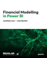
This book serves as a comprehensive guide to financial modeling, equipping readers with the skills and knowledge to create accurate, reliable models for analysis and decision-making. Designed for professionals, students, and finance enthusiasts, it bridges theoretical principles with practical Excel-based techniques, ensuring a balanced and thorough understanding of the subject.
Key Excel functions such as SUMPRODUCT, INDEX and MATCH, and LOOKUP are covered in depth, alongside essential tools like conditional formatting, data validation, and solver. The book emphasizes best practices in layout design, error checking, and model transparency, helping users build robust and easy-to-follow financial models. Practical methodologies for time-series analysis, control accounts, and financial statement theory are explored, making it a versatile resource.
The step-by-step model-building example guides readers through structuring, linking, and finalizing financial statements, including revenue, expenditure, taxation, and cash flow. Ratio analysis and self-review techniques are also discussed to ensure model accuracy and integrity. This detailed yet accessible guide empowers readers to create professional financial models with confidence and clarity.

Leseprobe

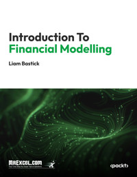
Introductionto Financial Modelling

How to Excel at Being a Lazy [That Means Efficient!] Modeller

FIRST EDITION

Dr. Liam Bastick

www.sumproduct.com

Copyright © 2018 SumProduct Pty Limited.

Published in 2018 by SumProduct Pty Limited.

Level 9, 440 Collins Street, Melbourne, Vic 3000, Australia.

All rights reserved.

No parts of this publication may be reproduced, stored in a retrieval system, or transmitted in any form or by any means, electronic, mechanical, photocopying, recording, scanning or otherwise, without either the prior written permission of the publisher, or authorisation through payment of the appropriate photocopy fee to the Copyright Clearance Center. Requests for permission should be addressed to the publisher, SumProduct Pty Limited, Level 9, 440 Collins Street, Melbourne, Vic 3000, Australia, tel: [phone], email: [email protected].

This publication is designed to provide accurate and authoritative information in regard to the subject matter covered. It is sold with the understanding that the publisher is not engaged in rendering public services. If professional advice or other expert assistance is required, the services of a competent professional person should be sought. SumProduct (www.sumproduct.com) is such an organisation that undertakes both tailored training and consulting services. Neither the author nor the publisher is liable for any actions prompted or caused by the information presented in this book. Any views expressed or implied herein are those of the author and do not represent the views of the organisations he works for.

Microsoft and Excel are registered trademarks of the Microsoft Corporation.

Published in the United States by Holy Macro! Books, PO Box 541731, Merritt Island FL 32953 ISBN 978-1-61547-066-2 (Print) 978-1-61547-152-2 (Digital)

About the Author

Dr. Liam Bastick FCA FCMA CGMA MVP

Starting off as a university lecturer, Liam has over 30 years’ experience in financial model development / auditing, valuations, M&A, strategy, training and consultancy. He has considerable experience in many different sectors (e.g. banking, energy, media, mining, oil and gas, private equity, transport and utilities and has worked in many countries including Australia, Belgium, Denmark, France, Germany, Hong Kong, Indonesia, Malaysia, New Zealand, Singapore, Switzerland, United States, United Kingdom and Vietnam, with many internationally recognised clients, constructing and reviewing strategic, operational and valuation models for many high profile International Public Offerings (IPOs), Leveraged Buyouts (LBOs) and strategic assignments.

With over 1,000 articles written for the accounting profession, he is a regular contributor to the American Institute of Certified Public Accountants (AICPA), Chartered Accountants Australia and New Zealand (CAANZ), Certified Practising Accountants Australia (CPAA), the Chartered Institute of Management Accountants (CIMA), the Institute of Chartered Accountants in England and Wales (ICAEW), Finance 3.0 and various LinkedIn specialist discussion groups. Liam is a Fellow of the Institute of Chartered Accountants (ICAEW), a Fellow of the Institute of Chartered Management Accountants (CIMA), a Chartered Global Management Accountant and is also a professional mathematician. Since 2012, he has been recognised by Microsoft as a Most Valuable Professional (MVP) in Excel, one of 104 such awardees worldwide (as at the time of writing).

Unfortunately, he follows Derby County and the England cricket team.

Preface

So, I finally managed it: I wrote this book. Over the years, like many of you, I have been frustrated about the content and detail of many texts supposedly on financial modelling. I’m a practitioner with 30 years’ experience and I kept seeing theoretical books that didn’t address the sorts of pragmatic issues that occur in reality.

Hence, I got off my backside and decided to do something about it. I have been writing in many accounting journals and on websites for years regarding common issues those working in in finance and forecasting face day in, day out. I decided it was time to go the whole hog and write a simple book on how to get started in financial modelling in such a way that you can easily have financial statements talking to each other and a Balance Sheet balancing readily and easily. It’s intended out for those starting on their journey to develop their modelling prowess and for more advanced users who are seeking a simpler way to put financial statements together, especially key practical tips and tricks to avoid the common pitfalls that bedevil the unwary.

I have been lucky enough to be appointed a Most Valuable Professional (MVP) by Microsoft for services to Excel - one of 104 so-recognised “experts” as at the time of writing. Now I know an “ex” is a has-been and a “spurt” is a drip under pressure, but I hope you’ll see me as a farmer - someone out(-)standing in their field! It takes thousands of mistakes to get good at something. This book is intended to show you how to avoid many of these traps.

I’d like to thank those that helped contribute to this book over the years (this has been 10 years in the making). Thanks to Bill Jelen for getting me to actually write it (even if we didn’t end up joining forces), Tim Heng for technically editing it and not deleting all my bad puns, Cecile Nguyen and Jonathan Liau for firming up the examples, and most importantly my immediate family, Nancy and little Layla, who have always supported me - even when I have gone many months spreading the word around the globe at the expense of a home life. To that end, I let my nine-year old daughter, Layla Bastick, have the last (fore)word:

“This book is a great source of information for people who are hoping to learn more about Excel and financial modelling. Liam Bastick has an amazing talent which helps people who read books like these to have a better understanding of modelling. This book is also inspiring for many of us thinking about becoming an expert in financial modelling or Excel. I am so proud of you daddy.”

Liam Bastick, March 2018

www.sumproduct.com

Editor’s notes

It’s entirely possible that I have spent more time than Liam did on this book - partly because he’s extremely good at what he does and condensed a lifetime of experience into a few weeks of furious book writing, and partly because I’ve spent a few minutes at every bit of humour that he’s written, wondering if we would be sued if I left it in. Suffice to say, you don’t need a PhD to see how the numbers work out there.

The challenge in writing a book about financial modelling is that the core of any modelling example is in the Excel files themselves. A picture may show a thousand words, but it’s incredibly hard to convey exactly how a formula or a set of calculations work without seeing the overall context of the model and being able to drill into the formula itself. With that in mind, we have set up a page on our website for further reference, where we will (for as long as our website and the internet as we know it still exists) provide files containing examples that we have used throughout this book, as well as any supplementary materials that we think may be useful: www.sumproduct.com/book-resources.

Although financial modelling has remained relatively consistent over the last few decades, there is always room for improvement, just as it is with this book. As with any text of this nature, there are bound to be typos, images that need improving, Excel features we’ve recommended that become deprecated, and new tips and ideas that demand to be included in the next edition of this book. Please let us know if you discover any errors, if you have any new ideas, or if you can think of better ways to present and explain the material that we have. We welcome any comments, best received via email at [email protected].

Tim Heng, Microsoft Excel MVP

www.sumproduct.com

Contents

Chapter 0: Introduction

Chapter 1: Key Excel Functions

1.1: SUM

1.2: IF

1.3: IFERROR

1.4: SUMIF

1.5: SUMIFS

1.6: SUMPRODUCT

1.7: VLOOKUP / HLOOKUP

1.8: LOOKUP

1.9: INDEX and MATCH

1.10: CHOOSE

1.11: OFFSET

1.13: EOMONTH and EDATE

1.14: MAX and MIN

Chapter 2: Key Excel Functionalities

2.1: Absolute Referencing

2.2: Number formatting

2.3: Styles

2.4: Conditional Formatting

2.5: Range Names

2.6: Data Validation

2.7: Data Tables

2.8: Goal Seek and Solver

2.9: Hyperlinks

Chapter 3: Best Practice Methodology

Chapter 4: Layout Tips

Chapter 5: Time Series Analysis

Chapter 6: Error Checks

Chapter 7: Model Template Example

Chapter 8: Financial Statement Theory

Chapter 9: Control Accounts

Chapter 10: Example Model Build

10.1: Initial Structure

10.2: Adding Sheets

10.3: Creating the Financial Statements

10.4: Linking the Financial Statement Worksheets .

10.5: Revenue

10.6: Costs of Goods Sold

10.7: Operating Expenditure

10.8: Capital Expenditure

10.9: Debt

10.10: Taxation

10.11: Equity

10.12: Single Entry Accounting

10.13: Opening Balance Sheet Revisited

10.14: Indirect Cash Flow Extract

10.15: Case Study Wrap-up

Chapter 11: Self Review

Chapter 12: Ratio Analysis

Appendix

Index

Chapter 0: Introduction

At last we meet.

I have been meaning to write this book for more years than I care to remember and you have decided that maybe there is a better way of building financial models that doesn’t involve trying to find Balance Sheet errors at 2am on a Saturday morning. It has always frustrated me that there’s never been a really practical book - heck, maybe a manual - that helps newcomers and the experienced alike to build better financial models. I just hope this one ticks some, if not all, of the boxes for you.

You may feel a little daunted looking at both the title and the thickness of this book. Hey, you’re worried - I’ve had to write this thing! For those of you unlucky enough to have met me, you’ll know I get bored very easily and you’ll also know I have a truly terrible sense of humour. Therefore, let’s make a pact: I am going to make this as easy and as practical a read as I can - and you’re going to tolerate my jokes. Deal..?

So what’s this book about? Well, I am going to assume that you, dear reader, have a basic understanding of Excel: I assume you are alive, you know how to open Excel, you know where the Ribbon is, you have used a keyboard before and that you can both read and type (sometimes even at the same time). I am also going to assume your work requires you to work in “finance” and that you have to work with financial projections or forecasts (most likely, you are charged with their preparation). This is who I am aiming this book at.

The plan is therefore as follows:

•Key Excel functions: Before we go anywhere, let’s do a refresher on the key functions most commonly required in financial modelling. That way, we are all on the same page. For the more advanced amongst you, may I suggest you read this section as well, as there’s stuff in here that many just don’t appreciate.

•Key Excel functionalities: There are other attributes that we need to take for granted too. In this section, I will discuss key functionalities such as absolute referencing, number formatting, conditional formatting, Data Tables, data validation, range names, hyperlinks and the like. OK, these features will be taken out of context, but it will make for an easier read when we talk about building the model.

•“Best Practice” methodology: There’s so much literature out there on this hotly-debated topic. Many academics and practitioners alike get hot under the collar just thinking about a model’s flexibility (maybe I could have phrased that better, but I did warn you about my sense of humour). I have even been involved in writing some of these said texts, but hey, I was young and I needed the money... However, we do need a conceptual framework and I propose something very simple - something I call CRaFT.

•Layout tips: Everyone always ploughs straight into Excel and seldom gives thought as to how to put a worksheet - never mind a workbook - together. Where should a heading go? Why? Should we use a convention for sheet tabs? Should we be pedantic about spacing? Citing units? Formatting? Copying? (The answer is yes; otherwise this will be a very short section.).

•Time series analysis: If we are going to build a model, we will have to work with dates - and that’s perhaps not quite as straightforward as you might think. In this section, I will explain how dates ought to be constructed and why - including periodicity issues - and where they should be positioned both in a worksheet and within the workbook to avoid errors.

•Error checks: Talking of errors, error checks are often added as an afterthought in a model. They shouldn’t be. In this section, I will explain why they should be at the forefront of your model development and implementation will just make your life - and the model user’s life - easier.

•Base template: No, I don’t mean, here’s a model I used last time and I will add a row here, delete a column there and deal with the #REF! errors and other model integrity issues when someone points them out to me. No; I accept all models are different, but they do share common attributes. It’s this foundation which I can translate into a base template to use at the outset of developing a financial model.

•Financial statement theory: It’s no secret that it was the phrases “double entry” and “working with models” that attracted me to this profession. How disappointed was I? On a serious note though, I want to revisit the key outputs of a financial model to fully understand what “three-way integrated” means and the ramifications for the modeller. Further, I actually go back to understand what is an Income Statement, a Balance Sheet and a Cash Flow Statement. Yes, you may know what they are - but I want to do it from the perspective of understanding the purpose of each statement so that it guides you in determining the order of building a financial model. No matter what you build, the derived order may be applied to all future model developments.

•Control accounts: How often have I mentioned debits and credits so far? Who said I haven’t? I just did in the first sentence. Debits and credits are the accountants’ way of keeping the mystery alive in finance. Hey, I think the bigger mystery more commonly encountered is, why doesn’t my Balance Sheet balance? If you choose to use control accounts, Balance Sheet errors will become a thing of the past.

•Example of a model build: Oh yes, might be an idea to actually build a model. This may be a small paragraph here, but it’s a big part of the book as we explain the four methods of model input, calculation tips etc. building in the order derived in the Financial statement theory section.

•Reviewing the model: Here, I talk about the difference between a “self-review” and a “model audit” and why the latter is very important. I present some common tips and tricks for checking your models - without any fancy add-in software - and even leave you with a suggested checklist and a discussion on ratio analysis.

Providing someone reads this book, future texts will cover “further reading”, such as what-if analysis, debt and the cash waterfall, valuations modelling and other corporate finance stories including mergers and acquisitions and project finance.

Before I proceed, let me stress one last thing: this book is a practical book. There are lots of supporting Excel models to play with and use, grouped by chapter / section, to visualise the important concepts discussed here. So no excuses, make sure you are sitting comfortably and open up Excel. There’s examples aplenty and the best way to understand is to do. Enjoy!

Chapter 1: Key Excel Functions

This chapter is dedicated entirely to going over the key functions most commonly used when developing a financial model in Excel. And you might be surprised regarding what’s on my shopping list:

•SUM

•SUMPRODUCT

•OFFSET

•IF

•VLOOKUP/HLOOKUP

•MOD

•IFERROR

•LOOKUP

•EOMONTH and EDATE

•SUMIF

•INDEX and MATCH

•MAX and MIN

•SUMIFS

•CHOOSE

Yes, they’re pretty straightforward: too often people show off using horror functions and formulae of length Tolstoy would have been proud. For me, financial modelling has one basic rule:

KEEP IT SIMPLE STUPID

That’s it. A colleague of mine once talked about the Rule of Thumb: Excel formulae in your formula bar should be no longer than your thumb:

I love this idea. It means the modeller - i.e. you - is forced into stepping out the logic making it easier for others to follow and more difficult for you to stuff up. I used to run a large Financial Model Audit team and I trained my staff to always be on the look-out for overly-complex formulae: the chances are the logic would contain errors and it may be that the model user might be trying to hide something too. Try not to fall into that trap.

OK, so with no further ado, let’s take a look at our function list in more detail.

CHAPTER 1.1: SUM

Is there really anyone out there that hasn’t encountered the SUM function? Given this book is intended to be about financial modelling rather than an introduction to Excel functions, is there anything new for me to tell you about SUM…?

Well, let me try.

SUM adds things up. It may include cells, numbers or ranges. In the context of financial modelling, summations are usually of numbers either directly above or to the left of the cell in question:

I use this all of the time in modelling. It’s a fast shortcut, it ensures you don’t miss cells within the range, it requires the range to be contiguous and you can’t leave blank cells. This shortcut actually forces you to build in a manner that will reduce the number of errors you might make. This reinforces one of my on-going themes:

A lazy modeller is to be encouraged; lazy modelling isn’t.

Let me be clear what I mean by a “lazy modeller”: this is someone who finds a way to keep formulae and constructs simple, so that their models are highly efficient and can be reproduced in seconds. It encourages flexibility, transparency and robustness - three key qualities of a “Best Practice” model (more on that later).

Lazy modelling may include typing in hard code, changing a formula on a cell by cell basis when it doesn’t quite work and refusing to add error checks to ensure model integrity. Lazy modelling always comes back to bite you. It may take longer initially to develop your model, but it will pay off many times over as the model continues to be used.

Be careful with SUM. Consider the following example:

In this example, I have totalled the values in cells E3:E7 in two distinct ways: the first uses the aforementioned SUM function with , the other has added each cell individually using the ‘+’ operator. Are you thinking you’d be mad to use the alternative (second) approach - especially if there were many more rows?

Well, take another look:

In this example, cell E5 has been modified. It has been stored as text, even though it looks like the number 3. SUM treats this as having zero value whereas the more convoluted addition carries on regardless. Simplest may not always be bestest.

In an example like the one above, this may be easy to spot, but would you stake your life that the sum here:

…is correct?

There is a simple way to check using the COUNT function. COUNT counts the number of numbers in a range, so we can use it to spot numbers that aren’t actually numbers:

Here, the formula in column I highlights when a number is not a number. Note how it reports by exception: if the cell in question contains a number then COUNT(Cell_Reference) equals 1 and 1-COUNT(Cell_Reference) equals zero. Only non-numbers will be highlighted - it’s better to know I have two errors rather than 14,367 values working correctly.

If you don’t think this applies to you, have you ever worked with PivotTables? This book isn’t about PivotTables, but as an aside, for those of you who have ever worked with this Excel feature, have you ever been frustrated when the following has happened?

You want your aggregation of values to default to SUM but instead they display as COUNT. This could be highlighting that some of your data is non-numerical and / or blank. Just a thought.

CHAPTER 1.2: IF

So what’s the most Important Function in Excel? Any takers for IF? The syntax for IF demonstrates just how useful this function is for financial modelling:

=IF(Logical_test,[Value_if_TRUE],[Value_if_FALSE])

This function has three arguments:

•Logical_test: this is the “decider”, i.e. a test that results in a value of either TRUE or FALSE. Strictly speaking, the Logical_test tests whether something is TRUE; if not, it is FALSE.

•Value_if_TRUE: what to do if the Logical_test is TRUE. Note that you do not put square brackets around this argument! This is just the Excel syntax for saying that this argument is optional. If this argument is indeed omitted, this argument will have a default value of TRUE.

•Value_if_FALSE: what to do if the Logical_test is FALSE (strictly speaking, not TRUE). If this argument is left blank, this argument will have a default value of FALSE.

This function is actually more efficient than it may look at first glance. Whilst the Logical_test is always evaluated, only one of the remaining two arguments is computed, depending upon whether the Logical_test is TRUE or FALSE. For example:

In this example, the intention is to evaluate the quotient Numerator / Denominator. However, if the Denominator is either blank or zero, this will result in an #DIV/0! error. Excel has several errors that it cannot evaluate, e.g. #REF!, #NULL, #N/A, #Brown, #Pipe. OK, so one or two of these I may have made up, but prima facie errors should be avoided in Excel as they detract from the key results and cause the user to doubt the overall model integrity. Worse, in some instances these errors may contribute to Excel crashing and / or corrupting. Note to self: prevent these errors from occurring.

This is where IF comes in. In my example above, =IF(Denominator=0,,Numerator/ Denominator) tests whether the Denominator is zero, If so, the value is unspecified (blank) and will consequently return a value of zero in Excel. Otherwise, the quotient is calculated as intended.

This is known as creating an error trap. Errors are “trapped” and the ‘harmless’ value of zero is returned instead. You could put “n.a” or “This is an error” as the Value_if_TRUE, but you get the picture.

It is my preference not to put a zero in for the Value_if_TRUE: personally, I think a formula looks clearer this way, but inexperienced end users may not understand the formula and you should consider your audience when deciding to put what may appear to be an unnecessary zero in a formula. The aim is to keep it simple for the end user.

An IF statement is often used to make a decision in the model, i.e.

=IF(Decision_Criterion=TRUE,Do_it,Don’t_Do_It)

This automates a model and aids management in decision making and what-if analysis. IF is clearly a very powerful tool when used correctly. However, sometimes it is used when another function might be preferable. For example, if you find yourself writing a formula that begins with:

=IF(IF(IF(IF…

then I humbly suggest you are using the wrong function. IF should never be used to look up data: there are plenty of functions out there to help with that problem, but we will come to that in time. However, sometimes your Logical_test might consist of multiple criteria, e.g.

=IF(Condition1=TRUE,IF(Condition2=TRUE,IF(Condition3=TRUE,1,),),)

Here, this formula only gives a value of 1 if all three conditions are true. This nested IF statement may be avoided using the logical function AND(Condition1,Condition2,…) which is only TRUE if and only if all dependent arguments are TRUE, i.e.

=IF(AND(Condition1,Condition2,Condition3),1,)

This is actually easier to read. There are two other useful logic functions sometimes used with IF:

•OR(Condition1,Condition2,…) is TRUE when at least one of the arguments is TRUE

•NOT(Condition) gives the opposite logic value, so that if the Condition is TRUE the result will be FALSE and vice versa.

Even using these logic functions, formulae may look complex quite quickly. There is an alternative: flags. In its most common form, flags are evaluated as

=(Condition=TRUE)*1

Flags make it easier to follow the tested conditions. Consider the following:

In this illustration, you might not yet understand what the MOD function does (more on that later), but hopefully, you can follow each of the flags in rows 4 to 7 without being an Excel guru. Row 9, the product, simply multiplies all of the flags together. This produces an AND flag. If I wanted the flag to be a 1 as long as one of the above conditions is TRUE (similar to OR), that is easy too:

Flags frequently make models more transparent and this example provides a great learning point. Often we mistakenly believe that condensing a model into fewer cells makes it more efficient and easier follow. On the contrary, it is usually better to step out a calculation. If it can be followed on a piece of paper (without access to the formula bar), then more people will follow it. If more can follow the model logic, errors will be more easily spotted. When this occurs, a model becomes trusted and therefore is of more value in decision-making.

I’d like to finish on a word of caution. Sometimes you just can’t use flags. Let me go back to my first example in this section - but this time using the flag approach:

Here, the flag does not trap the division by zero error. This is because this formula evaluates to

=#DIV/0! x 0

which equals #DIV/0! If you need to trap an error, you must use an IF function.

CHAPTER 1.3: IFERROR

IFERROR first came into being back in Excel 2007. It was something users had asked Microsoft for, for a very long time. But let me go back in time first and explain why.

At the time of writing, there are 12 IS functions, i.e. functions that give rise to a TRUE or FALSE value depending upon whether a certain condition is met:

1.ISBLANK(Reference): checks whether the Reference is to an empty cell

2.ISERR(Value): checks whether the Value is an error (e.g. #REF!, #DIV/0!, #NULL!). This check specifically excludes #N/A

3.ISERROR(Value): checks whether the Value is an error (e.g. #REF!, #DIV/0!, #NULL!). This is probably the most commonly used of these functions in financial modelling

4.ISEVEN(Number): checks to see if the Number is even

5.ISFORMULA(Reference): checks to see whether the Reference is to a cell containing a formula

6.ISLOGICAL(Value): checks to see whether the Value is a logical (TRUE or FALSE) value

8.ISNONTEXT(Value): checks whether the Value is not text (N.B. blank cells are not text)

9.ISNUMBER(Value): checks whether the Value is a number

10.ISODD(Number): checks to see if the Number is odd. Personally, I find the number 46 very odd, but Excel doesn’t

11.ISREF(Value): checks whether the Value is a reference

12.ISTEXT(Value): checks whether the Value is text.

You get the idea. As mentioned previously, sometimes you need to trap errors that may originate from a formula that is correct most of the time. Where possible, you should be specific with regard to what you are checking, e.g.

=IF(Denominator=0,Error_Trap,Numerator/Denominator)

In this example, I am checking to see whether the Denominator is zero. I could use this formula instead:

=IF(ISERROR(Numerator/Denominator),Error_Trap,Numerator/Denominator)

The difference here is that this will check for anything that may give rise to an error:

Do you see the problem here? I have to put the same formula in twice. If that is a long formula, then the calculation becomes doubly long. This is where IFERROR comes in; it halves the length of the calculation but still achieves the same effect:

=IFERROR(Calculation,Error_Trap)

Essentially, this formula is the bastard lovechild of IF and ISERROR. It checks to see whether the Calculation will give rise to a prima facie error. If it does, it will return Error_Trap; otherwise, it will perform the said Calculation, e.g.

You shouldn’t just sprinkle IFERROR throughout your models like your formulae are confetti. Used unwisely, IFERROR can disguise the fact that your formula isn’t working correctly and that modifications to the logic may be required. Try to use it sparingly.

Sometimes you have to use IF and ISERROR in combination anyway:

=IF(ISERROR(Calculation),Error_Trap,Different_Calculation)

In this example, the formula is checking to see whether a particular Calculation gives rise to an error. If it does, the Error_Trap will be referenced in the usual way, but if not a Different_ Calculation (not the Calculation used for the test) will be computed.

These two methodologies should be mastered. You will create more robust and flexible models once your error become a thing of the past. Not just the model - but your own expertise - will become more trusted in your organisation if users never encounter prima facie errors in your model.

CHAPTER 1.4: SUMIF

If you are unfamiliar with this function, you can still probably guess what SUMIF does: it combines SUM with IF to provide conditional summing, i.e. where you wish to add numerical values provided they meet a certain criterion. For example, imagine you were reviewing the following data summary:

The function SUMIF(Range,Criterion,Sum_range) is ideal for summing data based on one requirement:

•Range is the array that you wanted evaluated by the criterion (in this instance, cells F12:F21)

•Criterion is the criterion in the form of a number, expression, or text that defines which cell(s) will be added, e.g. “X”, 1, G26 or “<>“&G27 (this last one means “not equal to the value in cell G27”)

•Sum_range are the actual cells to be added if their corresponding cells in Range match the Criterion.

So, to find the sales for Business Unit 1 in the above example, you can use the formula =SUMIF(F12:F21,1,H12:H21) (which is $1,000), or to find the total sales of Product X, the formula could be modified to =SUMIF(G12:G21,”X”,H12:H21) (which is $1,200). Note that any text must be in inverted commas.

SUMIF is fine when there is only one condition. However, how would you find the total sales of Product Z in Business Unit 1 using this function? That’s two criteria and SUMIF does not work with multiple conditions. There are various alternatives using other functions, but it is possible to solve this problem simply using SUMIF.

It is often possible to cheat with SUMIF by making a ‘mega-criterion’ out of multiple criteria. This works on joining criteria together usually by using the ampersand (“&’) operator.

Let’s consider our example, slightly revised, from above.

A new column has been inserted (column H), with a formula combining the contents of columns F and G (e.g. the formula in cell H12 is =F12&G12). Provided that all possible combinations are unique (i.e. no duplicates can be generated), a simple SUMIF can then be applied, e.g.

=SUMIF(H12:H21,”1Z”,I12:I21).

This is by far and away the simplest solution - if it works. It can fall down though (in another example, the concatenation “111” might refer to Product 1 in Business Unit 11 or Product 11 in Business Unit 1).

As I say, there are other ways to solve this issue…

13

CHAPTER 1.5: SUMIFS

SUMIFS is similar to the SUMIF function. The syntax might not look similar when you first inspect it:

=SUMIFS(Sum_range,Criterion_range1,Criterion1,…)

If you think about it, the syntax is consistent with SUMIF. This function allows various ranges (Criterion_range1, Criterion_range2, …) to be assessed against multiple criteria (Criterionl, Criterion2, …). The key difference is that the range to be conditionally summed, Sum_range, is the first argument of the function rather than the last. This is so there is never any confusion regarding what is to be totalled.

Unlike the solution proffered in the SUMIF section, the helper column (column H) is no longer required. In some ways, this makes the function more straightforward, but it should remember that this function only arrived with the advent of Excel 2007 and therefore will not work with earlier versions of Excel.

There is another problem too - and this affects SUMIF as well. In fact, it’s an issue that harks back to our original discussion with the SUM function. SUM, SUMIF and SUMIFS have an Achilles’ Heel: numbers that look like numbers but are considered text (a common problem with data imported from management information systems) are treated as zero. This can lead to “right formula wrong result”:

There is only difference between this example and the previous one: cell I15 has now been entered as text. Therefore, the $400 is not recognised as a value and the summation has been reduced by this amount accordingly.

Care needs to be taken with these functions if conditional summations are to be relied upon in a financial model (the same may be said for PivotTables too).

But there’s a more robust alternative…

CHAPTER 1.6: SUMPRODUCT

I must admit this is one of my favourite functions in Excel - so much so our company was named after it (time for a shameless plug)!

At first glance,

SUMPRODUCT(Vector1,Vector2,…)

appears quite humble. Before showing an example, though, let’s look at the syntax carefully:

•A vector for Excel purposes is a collection of cells either one column wide or one row deep. For example, A1:A5 is a column vector, A1:E1 is a row vector, cell A1 is a unit vector and the range A1:E5 is not a vector (it is actually an array, but more on that later). The ranges must be contiguous; and

•This basis functionality uses the comma delimiter (,) to separate the arguments (vectors). Unlike most Excel functions, it is possible to use other delimiters, but this will be revisited shortly below.

So before I continue, I think it’s time to have a moan and reminisce about how I have been ripped off in the past. Just a couple of years ago, back when I was 18 (the Editor does not believe a word of this), I supported my studies by working at a petrol station. The hours were long (12 hours per day) and my boss would not buy an electronic till (yes, electricity had been invented back then), so all sales were recorded manually. Consequently, all sales had to be kept in a tally chart, i.e. the pricing points were listed in the first column and the sales were then noted in the second column. At the end of the day, I would have to calculate the total revenue and reconcile it with the payments received:

The sales in column H are simply the product of columns F and G, e.g. the formula in cell H12 is simply =F12*G12. Then, to calculate the entire amount cell H23 sums column H.

This could all be performed much quicker using the following formula:

=SUMPRODUCT(F12:F21,G12:G21)

i.e. SUMPRODUCT does exactly what it says on the tin: it sums the individual products.

I mentioned the comma delimiter earlier. You can multiply the vectors together instead.

=SUMPRODUCT(F12:F21*G12:G21)

will produce the same result. However, there is an important difference. If you think back to our earlier example:

SUMPRODUCT will work with numbers that aren’t really numbers. However, if you look at the formula in the example, you can be forgiven for not understanding the formula. Let me explain. Where SUMPRODUCT comes into its own is when dealing with multiple criteria. This is done by considering the properties of TRUE and FALSE in Excel, namely:

Consider the following example:

we can test columns F and G to check whether they equal our required values. SUMPRODUCT could be used as follows to sum only sales made by Business Unit 1 for Product Z, viz.

=SUMPRODUCT((F12:F21=1)*(G12:G21=“Z”)*H12:H21).

For the purposes of this calculation, (F12:F21=1) replaces the contents of cells F12:F21 with either TRUE or FALSE depending on whether the value contained in each cell equals 1 or not. The brackets are required to force Excel to compute this first before cross-multiplying.

Similarly, (G12:G21=“Z”) replaces the contents of cells G12:G21 with either TRUE or FALSE depending on whether the value “Z” is contained in each cell.

Therefore, the only time cells H12:H21 will be summed is when the corresponding cell in the arrays F12:F21 and G12:G21 are both TRUE, then you will get TRUE*TRUE*number, which equals the said number.

Note also that this uses the * delimiter rather than the comma, analogous to TRUE*number, etc. If you were to use the comma delimiter instead, the syntax would have to be modified thus:

=SUMPRODUCT(--(F12:F21=1),--(G12:G21=“Z”),H12:H21)

Minus minus? The first negation in front of the brackets converts the array of TRUEs and FALSEs to numbers, albeit substituting -1 for TRUE and 0 for FALSE. The second minus sign negates these numbers so that TRUE is effectively 1, rather than -1, whilst FALSE remains equals to zero. This variant often confuses end users which is why I recommend the first version described above.

You can get more sophisticated:

In this scenario, the end user pays invoices only where the invoice number matches the number “checked” on an authorised list. In the illustration above, two invoices (highlighted in red) do not match. SUMPRODUCT can be used to sum the authorised amounts only as follows:

=SUMPRODUCT((F12:F21=G12:G21)*H12:H21)

The argument in brackets only gives a value of TRUE for each row when the values in columns F and G are identical.

SUMPRODUCT and SUMIFS truly part company in the following comprehensive example. Consider the following:

So far, I have only considered SUMPRODUCT with vector ranges. Using the multiplication delimiter (*), it is possible to use SUMPRODUCT with arrays (an array is a range of cells consisting of both more than one row and more than one column).

In the above example, SUMPRODUCT has been used in its elementary form in cells I36:N36. For example, the formula in cell I36 is:

=SUMPRODUCT($H$32:$H$35,I$32:I$35)

and this has then been copied across to the rest of the cells.

To calculate the total costs of this retail bank example, this could be calculated as:

=SUMPRODUCT($I$36:$N$36,$I$21:$N$21)

However, the formula in cell I41 appears more - and unnecessarily - complicated:

=SUMPRODUCT($H$32:$H$35*$I$32:$N$35*$I$21:$N$21)

The use of the multiplication delimiter is deliberate (the formula will not work if the delimiters were to become commas instead). It should be noted that this last formula is essentially

=SUMPRODUCT(Column_Vector*Array*Row_Vector)

where the number of rows in the Column_Vector must equal the number of rows in the Array, and also the number of columns in the Array must equal the number of columns in the Row_Vector.

The reason for this extended version of the formula is in order to divide the costs between Budget and Standard costs in my example. For example, the formula in cell J41 becomes:

=SUMPRODUCT($H$32:$H$35*$I$32:$N$35*$I$21:$N$21*($G$32:$G$35=J$40))

i.e. the formula is now of the form

=SUMPRODUCT(Column_Vector*Array*Row_Vector*Condition)

where Condition uses similar logic to the TRUE / FALSE examples detailed earlier. This is a powerful concept that can be used to replace PivotTables for instance.

There are valid / more efficient alternatives to SUMPRODUCT in some instances. For example, dealing with multiple criteria for vector ranges, the SUMIFS function is up to six times faster, but will only work with Excel 2007 and later versions. Further, it cannot work with arrays where the dimensions differ such as in the example above.

Over-use of SUMPRODUCT can slow the calculation time down of even the smallest of Excel files, but it is a good all-rounder. Used sparingly it can be a highly versatile addition to the modeller’s repertoire. It is a sophisticated function, but once you understand how it works, you can start to use SUMPRODUCT for a whole array of problems (pun intended!).

CHAPTER 1.7: VLOOKUP/HLOOKUP

Often you will need to look up data in a table - and two functions most modellers are very familiar with are VLOOKUP and HLOOKUP. But do you realise it’s very easy to make a mistake with these functions? For those unsure of these functions, let me first start with a refresher.

VLOOKUP(Lookup_value,Table_array,Col_index_num,[Range_lookup])

has the following syntax:

•Lookup_value: What value do you want to look up?

•Table_array: Where is the lookup table?

•Col_index_num: Which column has the value you want returned?

•[Range_lookup]: Do you want an exact or an approximate match? This is optional and to begin with, I am going to ignore this argument exists.

HLOOKUP is similar, but works on a row rather than a column basis (horizontal rather than vertical).

I am going to use VLOOKUP throughout to keep things simple. VLOOKUP always looks for the Lookup_value in the first column of a table (the Table_array) and then returns a corresponding value so many columns to the right, determined by the Col_index_num column index number.

In this above example, the formula in cell G25 seeks the value 2 in the first column of the table F13:M18 and returns the corresponding value from the eighth column of the table (returning 47). Pretty easy to understand - so far so good. So what goes wrong? Well, what happens if you add or remove a column from the table range?

Adding gives us the wrong value:

With a column inserted, the formula contains hard code (8) and therefore, the eighth column (M) is still referenced, giving rise to the wrong value.

Deleting a column instead is even worse:

Now there are only seven columns so the formula returns #REF! Oops.

It is possible to make the column index number dynamic using the COLUMNS function:

COLUMNS(Reference) counts the number of columns in the Reference. Using the range F13:M13, this formula will now keep track of how many columns there are between the lookup column (F) and the result column (M). This will prevent the problems illustrated above.

But there’s more issues. Consider duplicate values in the lookup column. With one duplicate, the following happens:

Here, the second value is returned, which might not be what is wanted.

With two duplicates:

Ah, it looks like it might take the last occurrence. Testing this hypothesis with three duplicates:

Yes, there seems to be a pattern: VLOOKUP takes the last occurrence. I had better make sure:

Rats. In this example, the value returned is the fourth of five. The problem is, there’s no consistent logic and the formula and its result cannot be relied upon.

It gets worse if we exclude duplicates but mix up the lookup column a little:

In this instance, VLOOKUP cannot even find the value 2!

So what’s going on? The problem - and common modelling mistake - is that the fourth argument has been ignored:

VLOOKUP(Lookup_value,Table_array,Col_index_num,[Range_lookup])

[Range_lookup] appears in square brackets, which means it is optional. It has two values:

•TRUE: this is the default setting if the argument is not specified. Here, VLOOKUP will seek an approximate match, looking for the largest value less than or equal to the value sought. There is a price to be paid though: the values in the first column (or row for HLOOKUP) must be in strict ascending order - this means that each value must be larger than the value before, so no duplicates.

This is useful when looking up postage rates for example where prices are given in categories of kilograms and you have 2.7kg to post (say). It’s worth noting though that this isn’t the most common lookup when modelling.

•FALSE: this has to be specified. In this case, data can be any which way - including duplicates - and the result will be based upon the first occurrence of the value sought. If an exact match cannot be found, VLOOKUP will return the value #N/A.

And this is the problem highlighted by the above examples. The final argument was never specified so the lookup column data has to be in strict ascending order - and this premise was continually breached.

The robust formula needs both COLUMNS and a fourth argument of FALSE to work as expected:

This is a very common mistake in modelling. Using a fourth argument of FALSE, VLOOKUP will return the corresponding result for the first occurrence of the Lookup_value, regardless of number of duplicates, errors or series order. If an approximate match is required, the data must be in strict ascending order.

VLOOKUP (and consequently HLOOKUP) are not the simple, easy to use functions modellers think they are. In fact, they can never be used to return data for columns to the left (VLOOKUP) or rows above (HLOOKUP). So what should modellers use instead…?

CHAPTER 1.8: LOOKUP

Now that I have taken VLOOKUP and HLOOKUP to task, some of you may have considered LOOKUP is conspicuous by its absence. It may seem a less versatile function upon first glance, but it is quite useful for modelling. Allow me to explain.

LOOKUP has two forms: an array form and a vector form. As a reminder:

•An array is a collection of cells consisting of at least two rows and at least two columns

•A vector is a collection of cells across just one row (row vector) or down just one column (column vector).

The diagram should be self-explanatory:

The array form of LOOKUP looks in the first row or column of an array for the specified value and returns a value from the same position in the last row or column of the same array:

LOOKUP(Lookup_value,Array)

where:

•Lookup_value is the value that LOOKUP searches for in an array. The Lookup_value argument can be a number, text, a logical value, or a name or reference that refers to a value

•Array is the range of cells that contains text, numbers, or logical values that you want to compare with Lookup_value.

The array form of LOOKUP is very similar to the HLOOKUP and VLOOKUP functions.

The difference is that HLOOKUP searches for the value of Lookup_value in the first row, VLOOKUP searches in the first column, and LOOKUP searches according to the dimensions of array.

If Array covers an area that is wider than it is tall (i.e. it has more columns than rows), LOOKUP searches for the value of Lookup_value in the first row and returns the result from the last row. Otherwise, LOOKUP searches for the value of Lookup_value in the first column and returns the result from the last column instead.

The alternative form is the vector form:

LOOKUP(Lookup_value,lookup_vector,[result_vector])

The LOOKUP function vector form syntax has the following arguments:

•Lookup_value is the value that LOOKUP searches for in the first vector

•