Non-diffracting Waves E-Book
151,99 €
Mehr erfahren.
- Herausgeber: Wiley-VCH
- Kategorie: Wissenschaft und neue Technologien
- Sprache: Englisch
This continuation and extension of the successful book "Localized Waves" by the same editors brings together leading researchers in non-diffractive waves to cover the most important results in their field and as such is the first to present the current state.
The well-balanced presentation of theory and experiments guides readers through the background of different types of non-diffractive waves, their generation, propagation, and possible applications. The authors include a historical account of the development of the field, and cover different types of non-diffractive waves, including Airy waves and realistic, finite-energy solutions suitable for experimental realization. Apart from basic research, the concepts explained here have promising applications in a wide range of technologies, from wireless communication to acoustics and bio-medical imaging.
Sie lesen das E-Book in den Legimi-Apps auf:
Seitenzahl: 815
Veröffentlichungsjahr: 2013
Ähnliche


Table of Contents
Related Titles
Title Page
Copyright
Preface
List of Contributors
Chapter 1: Non-Diffracting Waves: An Introduction
1.1 A General Introduction
1.2 Eliminating Any Backward Components: Totally Forward NDW Pulses
1.3 Totally Forward, Finite-Energy NDW Pulses
1.4 Method for the Analytic Description of Truncated Beams
1.5 Subluminal NDWs (or Bullets)
1.6 “Stationary” Solutions with Zero-Speed Envelopes: Frozen Waves
1.7 On the Role of Special Relativity and of Lorentz Transformations
1.8 Non-Axially Symmetric Solutions: The Case of Higher-Order Bessel Beams
1.9 An Application to Biomedical Optics: NDWs and the GLMT (Generalized Lorenz-Mie Theory)
1.10 Soliton-Like Solutions to the Ordinary Schroedinger Equation within Standard Quantum Mechanics (QM)
1.11 A Brief Mention of Further Topics
Acknowledgments
References
Chapter 2: Localized Waves: Historical and Personal Perspectives
2.1 The Beginnings: Focused Wave Modes
2.2 The Initial Surge and Nomenclature
2.3 Strategic Defense Initiative (SDI) Interest
2.4 Reflective Moments
2.5 Controversy and Scrutiny
2.6 Experiments
2.7 What's in a Name: Localized Waves
2.8 Arizona Era
2.9 Retrospective
Acknowledgments
References
Chapter 3: Applications of Propagation Invariant Light Fields
3.1 Introduction
3.2 What Is a “Non-Diffracting” Light Mode?
3.3 Generating “Non-Diffracting” Light Fields
3.4 Experimental Applications of Propagation Invariant Light Modes
3.5 Conclusion
Acknowledgment
References
Chapter 4: X-Type Waves in Ultrafast Optics
4.1 Introduction
4.2 About Physics of Superluminal and Subluminal, Accelerating and Decelerating Pulses
4.3 Overview of Spatiotemporal Measurements of Localized Waves by SEA TADPOLE Technique
4.4 Conclusion
Acknowledgments
References
Chapter 5: Limited-Diffraction Beams for High-Frame-Rate Imaging
5.1 Introduction
5.2 Theory of Limited-Diffraction Beams
5.3 Received Signals
5.4 Imaging with Limited-Diffraction Beams
5.5 Mapping between Fourier Domains
5.6 High-Frame-Rate Imaging Techniques–Their Improvements and Applications
5.7 Conclusion
References
Chapter 6: Spatiotemporally Localized Null Electromagnetic Waves
6.1 Introduction
6.2 Three Classes of Progressive Solutions to the 3D Scalar Wave Equation
6.3 Construction of Null Electromagnetic Localized Waves
6.4 Illustrative Examples of Spatiotemporally Localized Null Electromagnetic Waves
6.5 Concluding Remarks
References
Chapter 7: Linearly Traveling and Accelerating Localized Wave Solutions to the Schrödinger and Schrödinger-Like Equations
7.1 Introduction
7.2 Linearly Traveling Localized Wave Solutions to the 3D Schrödinger Equation
7.3 Accelerating Localized Wave Solutions to the 3D Schrödinger Equation
7.4 Linearly Traveling and Accelerating Localized Wave Solutions to Schrödinger-Like Equations
7.5 Concluding Remarks
References
Chapter 8: Rogue X-Waves
8.1 Introduction
8.2 Ultrashort Laser Pulse Filamentation
8.3 The X-Wave Model
8.4 Rogue X-Waves
8.5 Conclusions
Acknowledgments
References
Chapter 9: Quantum X-Waves and Applications in Nonlinear Optics
9.1 Introduction
9.2 Derivation of the Paraxial Equations
9.3 The X-Wave Transform and X-Wave Expansion
9.4 Quantization
9.5 Optical Parametric Amplification
9.6 Kerr Media
9.7 Conclusions
Acknowledgments
References
Chapter 10: TE and TM Optical Localized Beams
10.1 Introduction
10.2 TE Optical Beams
10.3 Energetics of the TE Optical Beam
10.4 Discussion
10.5 Appendix
References
Chapter 11: Spatiotemporal Localization of Ultrashort-Pulsed Bessel Beams at Extremely Low Light Level
11.1 Introduction
11.2 Non-Diffracting Young's Interferometers
11.3 Non-Diffracting Beams at Low Light Level
11.4 Experimental Techniques and Results
11.5 Retrieval of Temporal Information
11.6 Wave Function and Fringe Contrast
11.7 Conclusions
Acknowledgments
References
Chapter 12: Adaptive Shaping of Nondiffracting Wavepackets for Applications in Ultrashort Pulse Diagnostics
12.1 Introduction
12.2 Space-Time Coupling and Spatially Resolved Pulse Diagnostics
12.3 Shack–Hartmann Sensors with Microaxicons
12.4 Nonlinear Wavefront Autocorrelation
12.5 Spatially Resolved Spectral Phase
12.6 Adaptive Shack–Hartmann Sensors with Localized Waves
12.7 Diagnostics of Ultrashort Wavepackets
12.8 Conclusions
Acknowledgments
References
Chapter 13: Localized Waves Emanated by Pulsed Sources: The Riemann–Volterra Approach
13.1 Introduction
13.2 Basics of the Riemann–Volterra Approach
13.3 Emanation from Wavefront-Speed Source Pulse of Gaussian Transverse Variation: Causal Clipped Brittingham's Focus Wave Mode
13.4 Emanation from a Source Pulse Moving Faster than the Wavefront: Droplet-Shaped Waves
13.5 Conclusive Remarks
References
Chapter 14: Propagation-Invariant Optical Beams and Pulses
14.1 Introduction
14.2 Theoretical Background
14.3 General Propagation-Invariant Solutions
14.4 Classification in Terms of Spectral and Angular Coherence
14.5 Stationary Propagation-Invariant Fields
14.6 Nonstationary Propagation-Invariant Fields
14.7 Conclusions
References
Chapter 15: Diffractionless Nanobeams Produced by Multiple-Waveguide Metallic Nanostructures
15.1 Introduction
15.2 Concept of Diffractionless Subwavelength-Beam Optics on Nanometer Scale
15.3 Diffractionless Nanobeams Produced by Multiple-Waveguide Metallic Nanostructures
15.4 Summary and Conclusions
Acknowledgments
References
Chapter 16: Low-Cost 2D Collimation of Real-Time Pulsed Ultrasonic Beams by X-Wave-Based High-Voltage Driving of Annular Arrays
16.1 Introduction
16.2 Classic Electronic Procedures to Improve Lateral Resolutions in Emitted Beams for Ultrasonic Detection: Main Limitations
16.3 An X-Wave-Based Option for Beam Collimation with Bessel Arrays
16.4 Low-Cost Circuits for Efficient Rectangular Driving of Annular Piezoelectric Transducerss
16.5 Comparative Excitation and Field Results Calculated for X-Beams
16.6 Conclusions
Acknowledgments
References
Chapter 17: Localized Beams and Localized Pulses: Generation Using the Angular Spectrum
17.1 Bessel Beams
17.2 The Bessel–Gauss Beam
17.3 Pulsed Bessel Beams
17.4 Applications in Biomedical Imaging
References
Chapter 18: Lossy Light Bullets
18.1 Introduction
18.2 Lossy Light Bullets in Self-Focusing Media with Nonlinear Losses
18.3 The Structured Profile of Lossy Light Bullets and their Energy Reservoir
18.4 Propagation Properties of Physically Realizable Lossy Light Bullets
18.5 Self-Reconstruction Property
18.6 Stability Properties
18.7 Conclusions
Acknowledgments
References
Chapter 19: Beyond the Diffraction Limit: Composed Pupils
19.1 Introduction
19.2 Theoretical Description
19.3 Super Resolving Pupils
19.4 Conclusions
Acknowledgments
References
Chapter 20: Experimental Generation of Frozen Waves in Optics: Control of Longitudinal and Transverse Shape of Optical Non-diffracting Waves
20.1 Introduction
20.2 Frozen Waves: Theoretical Description
20.3 Frozen Waves: Experimental Generation
20.4 Conclusions
Acknowledgments
References
Chapter 21: Airy Shaped Waves
21.1 Introduction
21.2 Airy Beams
21.3 Maximum Invariance Depth, Zmax
21.4 Analytical Description of Truncated Airy-Type Beams
21.5 Airy Pulses Considerations
21.6 Conclusions
Acknowledgments
References
Chapter 22: Solitons and Ultra-Short Optical Waves: The Short-Pulse Equation Versus the Nonlinear Schrödinger Equation
22.1 Introduction
22.2 Maxwell's Equations
22.3 Linear Propagation
22.4 Nonlinear Propagation: Instantaneous Nonlinear Response
22.5 Nonlinear Propagation: Time-dependent Nonlinear Response
22.6 Application: Mode-Locked Lasers
22.7 Conclusions
References
Index
Related Titles
Couairon, A., Mysyrowicz, A.
Nonlinear propagation of ultrashort laser pulses
From fundamentals to filamentation and self-focusing
2015
Print ISBN: 978-3-527-41186-3
Hernández-Figueroa, H.E., Zamboni-Rached, M., Recami, E. (eds.)
Localized Waves
2008
Print ISBN: 978-0-470-10885-7
The Editors
Prof. Hugo E. Hernández-Figueroa
University of Campinas
UNICAMP
School of Electrical and
Computer Engineering
Campinas, Brazil
Prof. Erasmo Recami
Universita Statale di Bergamo
Facolta di Ingegneria
Bergamo, Italy
Dr. Michel Zamboni-Rached
University of Campinas
UNICAMP
School of Electrical and
Computer Engineering
Campinas, Brazil
Cover figure
Copyright Hugo E. Hernández-Figueroa, Erasmo Recami, and Michel Zamboni-Rached.
All books published by Wiley-VCH are carefully produced. Nevertheless, authors, editors, and publisher do not warrant the information contained in these books, including this book, to be free of errors. Readers are advised to keep in mind that statements, data, illustrations, procedural details or other items may inadvertently be inaccurate.
Library of Congress Card No.: applied for
British Library Cataloguing-in-Publication Data
A catalogue record for this book is available from the British Library.
Bibliographic information published by the Deutsche Nationalbibliothek
The Deutsche Nationalbibliothek lists this publication in the Deutsche Nationalbibliografie; detailed bibliographic data are available on the Internet at <http://dnb.d-nb.de>.
© 2014 Wiley-VCH Verlag GmbH & Co. KGaA, Boschstr. 12, 69469 Weinheim, Germany.
All rights reserved. (including those of translation into other languages). No part of this book may be reproduced in any form — by photoprinting, microfilm, or any other means — nor transmitted or translated into a machine language without written permission from the publishers. Registered names, trademarks, etc. used in this book, even when not specifically marked as such, are not to be considered unprotected by law.
Print ISBN: 978-3-527-41195-5
ePDF ISBN: 978-3-527-67154-0
ePub ISBN: 978-3-527-67153-3
Mobi ISBN: 978-3-527-67152-6
oBook ISBN: 978-3-527-67151-9
Preface
Diffraction and dispersion effects are well known from centuries and are recognized to be limiting factors for many industrial and technological applications based, for example, on electromagnetic (EM) beams and pulses.
Diffraction is always present, affecting any waves that propagate in two-dimensional or three-dimensional (2D or 3D) media. Pulses and beams are constituted by waves traveling along different directions, which produces a gradual spatial broadening. This effect is a limiting factor whenever a pulse is needed, which maintains its transverse localization, for example, in free space communications, image forming, optical lithography, and EM tweezers.
Dispersion acts on pulses propagating in material media, causing mainly a temporal broadening; an effect due to the variation of the refraction index with the frequency, so that each spectral component of the pulse possesses a different phase-velocity. This entails a gradual temporal widening, which constitutes a limiting factor when a pulse is requested to maintain its time width, for example, in communication systems.
Consequently, the development of techniques capable of alleviating the signal degradation effects caused by these two effects is of crucial importance. Nondiffracting waves (NDWs), known also as localized waves, are indeed able to resist diffraction for a long distance. Today, NDWs are well established both theoretically and experimentally, and are having innovative applications not only in vacuum but in material (linear or nonlinear) media too, showing to be able to resist also dispersion. Moreover, the NDWs allow compensating even for effects such as attenuation. Indeed, in dispersing homogeneous media, it is possible for instance to construct pulses that simultaneously resist the effects of diffraction and dispersion; and, in absorbing homogeneous media, it is possible to construct beams that resist the simultaneous effects of diffraction and attenuation.
As expounded in this book, their potential applications are being intensively explored, always with surprising results, in fields such as microwaves, optics, acoustics, and are promising also in mechanics, geophysics, elementary particle physics, and gravitational waves. To confine ourselves to electromagnetism, let us mention the work on EM tweezers, optical (or acoustic) scalpels, optical guiding of atoms or (charged or neutral) corpuscles, optical lithography, optical images, communications in free space, remote optical alignment, optical acceleration of charged corpuscles, and so on. The NDWs are suitable superpositions of Bessel beams. (Let us recall in particular that a peculiar superposition of Bessel beams can be used to obtain “static” NDW fields, with high transverse localization, and whose longitudinal intensity pattern can assume any shape within a chosen interval of the propagation axis. Such beams, called “frozen waves” (FWs), have been experimentally produced in recent times in the case of optics as reported also in this book; they too promise to have very important applications, even in the field of medicine, for example, for tumor curing.)
Considering the significant amount of exciting and impressive results published in the recent 5 years or so, we decided to edit this book on this topic, after the first one appeared in 2008, published by John Wiley & Sons, Inc. These books are the first ones of their kind in the literature. The present volume is composed of 22 chapters authored by many of the worldwide most productive researchers in the field, with a balanced presentation between theory and experiments.
Chapter 1, by Recami et al., presents a thorough review of NDWs, emphasizing their theoretical foundations (in terms of exact solutions to the wave equations) along with historical aspects and the interconnections of this subject with other technological and scientific areas. It shows in particular how to eliminate any backward-traveling components (also known as noncausal components) in the case of both ideal and realistic finite-energy NDW pulses; and a method is then presented for an analytical description of truncated beams. The interesting case of the subluminal NDWs, or bullets, is moreover investigated, which leads to a new analytic description of FWs (endowed with a static envelope) in terms of continuous Bessel beam superpositions. The production of FWs is studied for absorbing media too. The role of special relativity and of Lorentz transformations, for the physical comprehension of the whole issue of NDWs, is stressed. Further topics are the use of higher order Bessel beams; an application to biomedical optics (by recourse to the generalized Lorenz–Mie theory); and, last but not least, the important fact that “soliton-like” solutions can be found also in the rather different case of the ordinary, linear Schrödinger equation within standard quantum mechanics.
Chapter 2 is authored by Ziolkowski, who coined the term “localized waves” and was involved with the topic at its inception. He reviews the initial years of focus wave modes, EM bullets, EM missiles, acoustic directed energy pulse trains (ADEPTs), electromagnetic directed energy pulse trains (EDEPTs), Bessel beams, complex beams, etc., until around the mid-1990s.
Chapter 3, by Mazilu and Dholakia, reviews theory, generation, properties, and applications of various nondiffracting beams, particularly the Bessel beam and Airy beams, and describes some emergent applications including imaging, micromanipulation, and cell transfection.
Chapter 4, by Saari, faces the circumstance that NDWs naturally became attractive to representatives of various fields, so that some misunderstandings showed up among the newcomers, for example, about nature, propagation velocity, and other properties of the NDWs. The first part of this chapter attempts to clarify issues such as the superluminal group velocity of X-type waves as opposed to their energy transport and signal velocity. It introduces the concept of superluminal accelerating and decelerating quasi-Bessel-X pulses, which are locally propagation-invariant. The second part of this chapter overviews experimental studies, where such a concept has been applied in time-domain treatment of diffraction of ultrashort light pulses on various apertures and optical elements.
Chapter 5, by J.-Y. Lu, deals with applications of limited-diffraction beams, such as X-waves, in high frame rate medical imaging. Various techniques related to such imaging method are introduced, including improvements of image quality and development of techniques for commercial realization of the method.
Chapter 6 is by Besieris and Shaarawi, who carefully discuss all the salient properties of spatiotemporally localized null EM waves (including their vortex structure, the Bateman constraint satisfied by them, and total energy and total angular momentum they carry). They show the Whittaker–Bateman potential theory to be a unifying approach for constructing wide classes of novel spatiotemporally localized luminal, superluminal, and hybrid null EM waves.
Chapter 7 is authored by Besieris, Shaarawi, and Ziolkowski. It aims at finding out a large class of nonsingular, localized, traveling wave solutions to the linear 3D Schrödinger equation, based on two interesting ansatzs. The second part of this chapter provides an account of a broad class of finite-energy accelerating localized wave solutions to the 3D Schrödinger equation, based on generalization of previous work on one-dimensional (1D) infinite-energy nonspreading wavepackets by Berry and Balazs.
In Chapter 8, Dubietis, Faccio, and Valiulis deal with the spontaneous formation of nonlinear X-waves, which is a known feature of intense ultrashort pulse propagation in transparent dielectrics (closely related to white-light continuum generation and femtosecond filamentation phenomena), and study the statistical aspects of the nonlinear X wave formation in presence of intensity, energy, and phase noise; meeting signatures of extreme events, that is, heavy-tailed statistical distributions. Such X-waves are interpreted as spatiotemporal optical rogue waves.
In Chapter 9, Conti shows how X-waves can be a basis for the second quantization of the optical field and how this approach enables to investigate nonlinear optical processes when employing highly nonmonochromatic beams. Implications on quantum entanglement and quantum information are discussed.
In Chapter 10, Hillion starts by recalling that the Helmholtz equation satisfied by the transverse electric (TE) and transverse magnetic (TM) fields (which is not the scalar Helmholtz equation) has elementary solutions in terms of Bessel and Hankel functions, and proves the existence of two different classes of solutions. He looks for solutions of the Helmholtz equation in the absence, or presence, of nonlinearities, showing, for example, that they are not of the Bessel type.
Chapter 11, by Bock and Grunwald, regards reflective axicons as modified, rotationally symmetric versions of the double slit setup, generating Bessel-like localized waves. Their experimental method works nondiffractively even for ultrashort pulses with large spectral bandwidths. They show how to reconstruct not only the spatial but also the temporal pulse information from quantum interference patterns formed by single photons; and introduce a spatiotemporal characterization of pulsed nondiffracting beams even at the quantum level (“quantum nondiffracting pulses”). Their results allow to exclude, incidentally, the interpretations of the double-slit experiment in which an interaction is assumed between separated slits (e.g., via surface plasmons). They finally propose a new method for a complete pulse reconstruction based on the nonlinear conversion of single photons from localized wavepackets.
Chapter 12 is authored by Bock et al. It shows that the arrays of free-space localized wavepackets allow an improved diagnostics of ultrashort pulses. In particular, the “needle pulses” can be used for analyzing the temporal properties of wavepackets with spatial resolution. The concept of needle beams is then extended toward more complex nondiffracting patterns. With reflective liquid-crystal-on-silicon-type spatial light modulators (SLMs), shaping and characterization of wavepackets at pulse durations down to 6 fs are demonstrated.
In Chapter 13, Utkin observes that the well-known frequency domain methods, for describing wave generation and propagation, disseminated the belief that a wave is something having a phase and an amplitude, rather than a solution of the wave equations. Although being complex and less universal, the space–time domain methods may be more adequate for solving wave propagation problems; for example, when the source term has complicated spatiotemporal structure. This chapter introduces a new space–time domain ansatz, calling into the play an inhomogeneous partial differential equation (PDE) of the hyperbolic type. In many practically important cases, the canonical PDE has a known Riemann function, which makes possible to construct the unique solution to the above initial value problem harnessing the Riemann–Volterra formula. The applicability of the method for causal description of launching localized waves by physically admissible sources is demonstrated for two practically important cases: generation of a finite-support focus wave mode by a luminal-speed pulse with the Gaussian transverse variation, and launching of a droplet-shaped wave by a line source traveling with a superluminal speed.
Chapter 14, by Saastamoinen, Friberg, and Turunen, overviews a wide class of optical fields, which possess the same spectral density distribution across every plane perpendicular to the nominal propagation direction. Examples are given for both stationary and nonstationary fields with different spatial and temporal coherence properties. The simplest special cases include sharply peaked Bessel fields, Bessel-correlated fields, and localized wave packets, such as X-waves and focus wave modes.
Chapter 15, by Mechler and Kukhlevsky, shows–using the scalar diffraction theory and the image method–how any arbitrary scalar field, confined by a 2D or 3D optical waveguide, can be generated in free space by the appropriate light source. The correspondence between the guided and free-space waves is illustrated using several particular fields, such as the diffraction-free, self-imaging, ultra-short, soliton-like, partially coherent waves, and laser fractals.
Chapter 16, by Ramos, Castellanos, and Callás, starts referring to the experimental production of X-shaped acoustic waves by Lu et al. in 1992, which was based on the sequential excitations of annular array rings and subsequent synthesis by software composition. Its extension for a strict real-time regime would need an expensive, fast instrumentation with parallel electronic channels; however, fast beam synthesis is actually required in ultrasonic applications for medical diagnosis by imaging or noninvasive inspection in quality control. In this chapter, principles and implementation details are described for achieving real-time radiation of localized ultrasonic beams in pulsed regime, in such a way to achieve efficient implementations of fast X-beam collimations in the megahertz range at a low cost, for the multichannel electronics involved. A real-time ultrasonic emitting and beam-forming experiment in laboratory is described in detail. Optimization results for the annuli emissions and acoustic beam-forming patterns, from a specially designed piezoelectric annular array, are also compared with those obtained using the ideal zero-order X-wave solutions proposed in the classical approach by Lu et al.; and a very acceptable approximation level is obtained.
Chapter 17 is authored by Sheppard. It starts from pulsed beams generated by coherent superposition of Bessel beams. They can be compared among themselves using 3D (generalized) pupils. Applications in microscopy and tomography are discussed.
In Chapter 18, Porras reviews the properties of lossy light bullets; an alternative form of light wave localization in nonlinear media with dissipation (which is between a soliton and a conical wave). Unlike well-known dissipative light bullets, lossy light bullets do not require a continuous gain to sustain stationary propagation. Lossy light bullets are self-healing and are stabilized by losses, which make them attract the self-focusing dynamics in dissipative media.
Chapter 19, by Ranfagni and Mugnai, recalls how in 1952 Toraldo di Francia proposed an intriguing method to increase the optical resolving power. His theory might seem to be in contradiction with Heisenberg's uncertainty correlations. In this chapter, the authors report the results of microwave investigations, which demonstrate the correctness of that theoretical prediction and its interpretation in relation to the uncertainty principle. Experimental measurements, employing special composed pupils, have been made in order to verify the possibility of obtaining a considerable reduction in the beam width and a field concentration along the axial axis, as compared to a simple pupil. Further experiments have been devoted to evaluate the pulse delay in the propagation, in the presence of this kind of pupils.
Chapter 20, by Vieira, Gesualdi, and Zamboni-Rached, presents, for the first time, the experimental generation of FWs in optics, obtained using a setup for the optical reconstruction of computer-generated holograms (CGHs), based on a 4-F Fourier filtering system and a nematic liquid crystal spatial light modulator (LC-SLM). The CGHs have been implemented computationally and, subsequently, electronically in the LC-SLM for optical reconstruction. The results agree with the corresponding theoretical (analytic) solutions and bear excellent perspectives for scientific and technological applications.
Chapter 21 is authored by Nóbrega, Dartora, and Zamboni-Rached. It presents an analytic method for the description of Airy-type beams when truncated by finite apertures: a method based on suitable superposition of exponentially decaying Airy beams. The results can be quickly evaluated via the simple analytic solution proposed in this chapter, and agree with those obtained in the literature through numerical methods. Three different truncated beams are analyzed: ideal Airy, Airy-Gauss, and Airy-exponential beams.
Chapter 22, by Kutz, deals with sources of ultrashort light pulses, which enable direct observation of some of the fastest processes in nature, along with studies of matter under extreme conditions (leading to the first studies of the hitherto unexplored field of attosecond physics). It envisions that even single-electron transition events can now be captured. The theoretical models, however, have lagged behind because of their adherence to standard center-frequency expansion techniques for modeling the electric field envelope in Maxwell's equations; whereas below a few femtosecond regimes such theories begin to breakdown and new approaches must be developed. In this chapter, a mode-locking theory is developed, which is valid in the ultrashort pulse regime, the starting point being Maxwell's equations. When pushed to the extreme of a few femtoseconds or attosecond pulses, even the so-called nonlinear Schrödinger equation (NLS) description becomes suspect. Thus, a simplified approach is taken in this chapter, where the description of the pulse is derived directly from Maxwell's equations. Specifically, a mode-locking in a laser cavity is considered, taking advantage of the robust and stable mode-locking that results in the short-pulse limit.
Preparation of this book's manuscript was greatly facilitated by Anja Tschoertner, Aarthi Elumalai, and George J. Telecki from Wiley Publishers. We thank them for their fine, friendly, and professional work. The authors, all of them among the world leaders in this field, contributed always enthusiastically in a very efficient manner; we thank in particular Richard W. Ziolkowski, a pioneer in the field. We are also very indebted to Kai Chang, as well as Claudio Conti, and Daniele Faccio, for inspirational encouragement or help.
July 2013
Hugo E. Hernández-Figueroa
Erasmo Recami
Michel Zamboni-Rached
List of Contributors
1
Non-Diffracting Waves: An Introduction1
Erasmo Recami, Michel Zamboni-Rached, Hugo E. Hernández-Figueroa, and Leonardo A. Ambrosio
1.1 A General Introduction
1.1.1 A Prologue
In this chapter, which essentially deals with exact solutions to the wave equations, we begin by introducing the topic of non-diffracting waves (NDW), including some brief historical remarks, and by a simple definition of NDWs; afterward we present some recollections – besides of ordinary waves (Gaussian beams, Gaussian pulses) – of the simplest NDWs (Bessel beams, X-shaped pulses, etc.). More details can be found in the first two (introductory) chapters of the volume on Localized Waves published [1] in 2008. In section 1.2 we go on to show how to eliminate any backward-traveling components (also known as non-causal components), first in the case of ideal NDW pulses, and then, in section 1.3, for realistic, finite-energy NDW pulses. In particular, in section 1.3.1 we forward a general functional expression for any totally-forward non-diffracting pulses. Then, in section 1.4 an efficient method is set forth for the analytic description of truncated beams, a byproduct of its being the elimination of any need of lengthy numerical calculations. In section 1.5 we explore the not-less-interesting question of the subluminal NDWs, or bullets, in terms of two different methods, the second one being introduced as it allows the analytic description of NDWs with that is of NDWs with a static envelope (“frozen waves” (FW)) in terms of continuous Bessel beam superpositions. The production of such FWs (which, indeed, have been generated experimentally in recent time for optics) is developed theoretically in section 1.6 also for the case of absorbing media. Section 1.7 discusses the role of special relativity and of Lorentz transformations (LTs), which is relevant for the physical comprehension of the whole issue of NDWs. In section 1.8 we present further analytic solutions to the wave equations, with use of higher-order Bessel beams (namely, non-axially symmetric solutions). Next, section 1.9 deals in detail with an application of NDWs to biomedical optics by having recourse to the generalized Lorenz–Mie theory (GLMT). In section 1.10 we exploit the important fact that “soliton-like” solutions can be found also in the rather different case of the ordinary, linear Schroedinger equation – which is not a properly said wave equation – within standard quantum mechanics; by also constructing, for instance, a general exact non-diffracting solution for such equation. These “localized” solutions to the Schroedinger equation may a priori be of help for a better understanding, say, of de Broglie's approach and of the particle-wave duality. Some complementary issues are mentioned in the last section.
Let us now start by recalling that diffraction and dispersion are long-known phenomena limiting the applications of beams or pulses.
Diffraction is always present, affecting any waves that propagate in two or three-dimensional (3D) media. Pulses and beams are constituted by waves traveling along different directions, which produces a gradual spatial broadening. This effect is a limiting factor whenever a pulse is needed, which maintains its transverse localization, like, for example, in free space communications, image forming, optical lithography, and electromagnetic tweezers, etc.
Dispersion acts on pulses propagating in material media causing mainly a temporal broadening, an effect due to the variation of the refraction index with the frequency, so that each spectral component of the pulse possesses a different phase velocity. This entails a gradual temporal widening, which constitutes a limiting factor when a pulse is needed that maintains its time width, like, for example, in communication systems.
It has been important, therefore, to develop techniques able to reduce those phenomena. NDW, known also as localized waves, are, indeed, able to resist diffraction for a long distance. Today, NDW are well-established both theoretically and experimentally, and have innovative applications not only in vacuum, but also in material (linear or nonlinear) media, also showing resistance to dispersion. As mentioned, their potential applications are being explored intensively, always with surprising results, in fields like acoustics, microwaves, and optics, and are also promising in mechanics, geophysics [2], and even elementary particle physics [3] and gravitational waves. One interesting acoustic application has been already obtained in high-resolution ultra-sound scanning of moving organs in the human body. We shall see that NDWs are suitable superpositions of Bessel beams. And worth noticing is that peculiar superposition of Bessel beams can be used to obtain “static” NDW fields, with high transverse localization, and whose longitudinal intensity pattern can assume any desired shape within a chosen interval of the propagation axis; such waves with a static envelope [1, 4–7], that we called FW, have been produced experimentally in recent times in the case of optics, as reported elsewhere also in this book. These FWs promise to have very important applications (even in the field of medicine and of tumor curing [8]).
To confine ourselves to electromagnetism, let us recall again the present-day studies on electromagnetic tweezers, optical (or acoustic) scalpels, optical guiding of atoms or (charged or neutral) corpuscles, optical lithography, optical (or acoustic) images, communications in free space, remote optical alignment, optical acceleration of charged corpuscles, and so on.
1.1.2 Preliminary, and Historical, Remarks
Ordinary beams and pulses are superpositions of plane waves that travel in different directions; this causes diffraction and, consequently, an increasing spatial broadening of the waves during propagation. Incidentally, we are considering here only propagating, that is non-evanescent, waves.
Surprisingly, solutions to the wave equations exist, which represent in homogeneous media beams and pulses able to resist the effects of diffraction for long distances. Such solutions are called NDW, or localized waves (LW); even if a better name would be “limited-diffractions waves” [9, 10].
The theory of NDWs also allows compensating for effects like dispersion and attenuation. Indeed, in dispersing homogeneous media, it is possible to construct pulses that simultaneously resist the effects of diffraction and of surface dispersion. And, in absorbing homogeneous media, it is also possible to construct beams that resist the simultaneous effects of diffraction and of attenuation.
For earlier reviews about NDWs, we refer the reader, for instance, to the first two chapters of the Localized Waves [1], as well as Advances in Imaging and Electron Physics [11], and references therein. There, the reader will find general and formal (simple) introductions to NDWs, with more details on the separate cases of beams and of pulses, as well as on the rather different characteristics of the Bessel and of NDWs, with respect to (w.r.t.) the Gaussian ones. The important properties of the former w.r.t. the latter ones can find application, as well-known and as stressed therein, in all fields in which an essential role is played by a wave–equation (e.g., electromagnetism, optics, acoustics, seismology, geophysics, and also gravitation, and elementary particle physics).
Here, let us only insert the following, quite brief historical information.
The non-diffracting solutions to the wave equations (scalar, vectorial, spinorial etc.) have been in fashion, both in theory and in experiment, for a couple ofdecades. Rather well known are the ones with luminal or superluminal peak-velocity [1] like the so-called X-shaped waves (see [9, 12, 13] and references therein), which are supersonic in acoustics [10], and superluminal in electromagnetism (see [14]; see also [15] and [16]).
It has already been recognized by Bateman [17] and later on Courant and Hilbert [18], that luminal NDWs exist, which are solutions to the wave equations. After subsequent early works, already quoted by us, a great deal of results [19] have been published on NDWs, from both the theoretical and the experimental point of view: initially, taking only free space into account, and, later on, considering more complex media, which exibit effects such as dispersion (see, e.g. [20–22]), nonlinearity [23], anisotropy [24–26], losses [5], and so on. Extensions of this type have been carried out along with the development, for instance, of efficient methods for obtaining non-diffracting beams and pulses in the subluminal, luminal, and superluminal regimes, thus allowing easier experimental verifications.
Indeed, in recent years, some attention [19, 27–33] started to be paid to the (more “orthodox”) subluminal NDWs, too. It should be stressed that, in any case, the interest in NDWs resides not in their peak-velocity [34–36] but in that they propagate in a homogeneous linear medium without distortion – and in a self-reconstructing way [5, 37, 38] (apart from local variations, in the sense that their square magnitude keeps its shape during propagation, while local variations are shown only by its real, or imaginary, part).
In the past, however, little attention was paid to Brittingham's 1983 paper [39], wherein he obtained pulse-type solutions to the Maxwell equations, which propagated in free space as a new kind of -speed “solitons.” That lack of attention was partially due to the fact that Brittingham had neither been able to get finite-energy expressions for his “wavelets” nor to make suggestions about their practical production. Two years later, however, Sezginer [40] was able to obtain quasi-non-diffracting luminal pulses endowed with a finite energy: Finite-energy pulses are known not to travel undistorted for an infinite distance, but nevertheless propagate without deformation for a long field-depth, much larger than the one achieved by ordinary pulses like the Gaussian ones (see, e.g., [41–52] and references therein).
An interesting problem, indeed, was that of investigating what would happen to the ideal Bessel beam solution when truncated by a finite transverse aperture. In 1987 a heuristical answer was found after the quoted series of pioneering papers [41–44] from the experiments by Durnin et al. [45, 46], when it was shown that a realistic Bessel beam, passing through a finite aperture, is able to travel keeping its transverse intensity shape approximately unchanged all along a large “depth of field.”
In any case, only after 1985 a general theory of NDWs started to be extensively developed [9, 12, 14, 53–65], both in the case of beams and in the case of pulses. For reviews, see, for instance [1, 11, 13, 48, 50–52, 61] and references within. For the propagation of NDWs in bounded regions (like wave-guides), see [66–68] and references therein. For the focusing of NDWs, see, for example [1, 69, 70], and references therein. For recourse to chirped optical X-type waves to obtain pulses capable of recovering their spatial shape both transversally and longitudinally, see, for example, [1, 71] and references therein. Not less important, for the construction of general NDWs propagating in dispersive media, see, besides the quoted [20–22], also [72–74]; while, for lossy media, see, for example [1, 5, 69, 70] and references therein, and this chapter. Finally, for finite-energy, or truncated, solutions see, for example, [57, 75–79] as well as this chapter.
NDWs have now been produced experimentally [10, 80–83], and are being applied in fields ranging from ultrasound scanning [30, 33, 77, 84] to optics (for the production, e.g., of new type of tweezers [5, 8, 85–87]). All those works have demonstrated that non-diffracting pulses can travel with any arbitrary peak-velocities υ, that is with speed υ in the range .
Let us introduce at this point a first mathematical definition of NDWs.
Diffraction, as a spatial transverse spreading, cannot occur in the simple case of one space dimension (1D). Actually, the 1D wave equation
1.1
admits the general solution , quantities and being arbitrary(differentiable) functions; and, for instance, a solution of the type travels rigidly along the positive -direction with speed . Let us here recall, and stress, that if a wave depends on and only through the quantity , it will be seen as moving without any distortion with the speed : see, for example [13], and references therein.
Moving on to the 3D case, when the wave equation reads
1.2
quantity being the transverse Laplacian, and the transverse position vector (so that ), it is natural to look for possible solutions of the type
1.3
which would correspond to waves rigidly propagating along with speed , whatever the value of is (see [1, 13]). To check the mentioned possibility, let us go back to Equation 1.2. It is simple to show, then, that an acceptable solution of the type 3 has just to satisfy the equation
1.4
where . (Let us explicitly repeat and recall [50] that the shape of any solutions that depend on and on only through the quantity will always appear the same to an observer traveling along with the speed , whatever be (subluminal, luminal, or superluminal) the value of ; that is, such a solution will propagate rigidly with speed .]
One can therefore realize the following:
The latter simple and interesting result shows that, when basing ourselves on Equation 1.4, the solutions that can propagate rigidly (i.e., without any spatial modifications) are those corresponding to . In the case of beams, is merely the phase velocity; but, in the case of pulses it is the peak velocity (sometimes identified with the group-velocity). Incidentally, it is known that, when one superposes waves whose phase-velocity does not depend on their frequency, such a phase-velocity becomes2 the actual peak-velocity [50, 67, 88].
Many interesting solutions of this kind exist [1, 9, 10, 14, 57], and some of them will be mentioned in this chapter, and in this very book. From a historical point of view, let us repeat that such solutions to the wave equations (and, in particular, to the Maxwell equations, under weak hypotheses) were predicted theoretically a long time ago [17, 18, 89, 90], mathematically constructed in more recent times [9, 14, 91], and, soon after, produced experimentally [10, 80–83].
However, it is rather restrictive to define a NDW as a solution of the type 3, with. Actually, subluminal NDW solutions to the wave equations also exist [19], and they, too, are rather interesting, as we shall discuss below.
1.1.3 Definition of Non-Diffracting Wave (NDW)
Therefore, it is convenient to formulate a more comprehensive definition, wherefrom to derive a much ampler set of solutions (superluminal, luminal, or subluminal) capable of withstanding diffraction, both for infinite distances, in the ideal case (of infinite energy), and for large, but finite distances, in the realistic case (of finite energy).
Let us start by formulating an adequate definition of an ideal NDW.
Let us consider a linear and homogeneous wave equation in free space. In cylindrical coordinates and using a Fourier–Bessel expansion, its general solution can be expressed, when disregarding evanescent waves, as
1.5
with
1.6
the being arbitrary functions, and the Dirac delta function. It is important to emphasize that the are -order Bessel functions. For simplicity, many authors often confine themselves to the zero-order Bessel functions .
An ideal NDW is a wave that must be capable of maintaining indefinitely its spatial form (except for local variations) while propagating. This property may be mathematically expressed, when assuming propagation in the -direction, as follows:
1.7
where is a chosen length, and is the pulse-peak velocity, with . Then, by using Equation 1.5 into Equation 1.7, and taking account of Equation 1.6, one can show [1, 12, 63] that any non-diffracting solution can be written as
1.8
with
1.9
where (with an integer number too, of course), while quantity is an arbitrary frequency spectrum. Notice that, owing to Equation 1.9, each term in the double sum (1.8), namely in its expression within square brackets, is a truly NDW (beam or pulse); and their sum (1.8) is just the most general form representing an ideal NDW according to definition 1.7.
One should also notice that (1.8) is nothing but a superposition of Bessel beams with a specific “space–time coupling,” characterized by linear relationships between their angular frequency and their longitudinal wave number .
Concerning such a superposition, the Bessel beams with () propagate in the positive (negative) -direction. As we wish to obtain NDWs propagating in the positive -direction, the presence of “backward” Bessel beams is not desirable, that is, of “backward components” – often called non-causal, as they should be entering the antenna or generator. The problems with the backward-moving components, that so frequently plague the localized waves, can be overcome, however, by appropriate choices of the spectrum (1.9), which can totally eliminate those components, or minimize their contribution, in superposition (1.8). Let us notice that often only positive values of are considered ().
Another important point refers to the energy [12, 40, 52, 92] of the NDWs. It is well known that any ideal NDW, that is, any field with the spectrum (1.9), possesses infinite energy. However, finite-energy NDWs can be constructed by concentrating the spectrum in the surrounding of a straight line of the type instead of collapsing it exactly over that line [12, 63]. In such a case, the NDWs get a finite energy, but, as we know, are endowed with finite field depths, that is, they maintain their spatial forms for long (but not infinite) distances.
Despite the fact that expression 1.8, with given by Equation 1.9, does represent ideal NDWs, it is difficult to use it for obtaining analytical solutions, especially when there is the task of eliminating the backward components. This difficulty becomes even worse in the case of finite-energy NDWs. We shall come back to this point in section 1.2.
1.1.4 First Examples
Before going on, let us be more concrete. First of all, let us notice that Equation 1.5, for and on integrating over , reduces to the less general – but still quite useful – solution
1.10
where is now the chosen spectral function, with only (and we still disregard evenescent waves). We are using the standard relation
1.11
From the integral solution (1.10) one can get in particular, for instance, the (non-localized) Gaussian beams and pulses, to which we shall refer for illustrating the differences of the NDWs w.r.t. them.
The Gaussian beam is a very common (non-localized) beam [93], corresponding to the spectrum
1.12
In Equation 1.12, is a positive constant, which will be shown to depend on the transverse aperture of the initial pulse.
The integral solution (1.10), with spectral function (1.12), can be regarded as a superposition of plane waves: namely, of plane waves propagating in all directions (always with kz ≥ 0), the most intense ones being those directed along (positive) z (especially when ). This is depicted clearly in Figure 1.4 of [1].
On substituting Equation 1.12 into Equation 1.10and adopting the paraxial approximation (which is known to be just valid if ), one meets the Gaussian beam
1.13
where . We can verify that the magniture of such a beam, which suffers transverse diffraction, doubles its initial width after having traveled the distance , called the diffraction length. The more concentrated a Gaussian beam happens to be, the more rapidly it gets spoiled.
The most common (non-localized) pulse is the Gaussian pulse, which is obtained from Equation 1.10 by using the spectrum [71]
1.14
where and are positive constants. Indeed, such a pulse is a superposition of Gaussian beams of different frequency.
Now, on substituting Equation 1.14 into Equation 1.10, and adopting once more the paraxial approximation, one gets the Gaussian pulse:
1.15
endowed with speed and temporal width , and suffering a progressing enlargement of its transverse width, so that its initial value gets doubled already at position , with . Let us remember that the paraxial approximation is really valid in the pulse case only if there hold the two conditions and , imposing a slow variation of the envelope.
1.1.5 Further Examples: The Non-Diffracting Solutions
Let us finally go on to the construction of the two most renowned localized waves [48]: the Bessel beam and the ordinary X-shaped pulse. First of all, let us recall that, when superposing (axially symmetric) solutions of the wave equation in the vacuum, three spectral parameters,, come into the play, which have, however, to satisfy the constraint (1.11), deriving from the wave equation itself. Consequently, only two of them are independent, and we here choose and . Such a possibility of choosing and was already apparent in the spectral functions generating Gaussian beams and pulses, which consisted of the product of two functions, one depending only on and the other on .
We are going to see that further particular relations between and (or, analogously, between and ) can be enforced in order to get interesting and unexpected results, such as the NDWs.
Let us start by imposing a linear coupling between and (it could, actually be shown [46] that it is the unique coupling leading to NDW solutions).
Namely, let us consider the spectral function
1.16
which implies that , with : a relation that can be regarded as a space–time coupling. Let us add that this linear constraint between and , together with relation 1.11, yields . This is an important fact, as an ideal NDW must contain [12, 48] a coupling of the type , where and are arbitrary constants. The integral function 1.10, this time with spectrum (1.16), can be interpreted as a superposition of plane waves; however, this time the axially-symmetric Bessel beam appears as the result of the superposition of plane waves whose wave vectors lay on the surface of a cone having the propagation line as its symmetry axis and an opening angle equal to; such being called the axicon angle. This is shown clearly in Figure 1.5 of [1].
By inserting Equation 1.16 into Equation 1.10, one gets the mathematical expression of the so-called Bessel beam:
1.17
This beam possesses phase-velocity , and field transverse shape represented by a Bessel function so that its field is concentrated in the surroundings of the propagation axis . Moreover, Equation 1.17 tells us that the Bessel beam keeps its transverse shape (which is therefore invariant) while propagating, with central “spot” .
The ideal Bessel beam, however, is not square-integrable in the transverse direction, and is therefore associated with an infinite power flux, that is, it cannot be produced experimentally. One must have recourse to truncated Bessel (TB) beams, generated by finite apertures: In this case the (truncated) Bessel beams are still able to travel a long distance while maintaining their transfer shape, as well as their speed, approximately unchanged [45, 46, 94, 95]. For instance, the field-depth of a Bessel beam generated by a circular finite aperture with radius is given (if ) by
1.18
where is the beam axicon angle. In the finite aperture case, the Bessel beam can no longer be represented by Equation 1.17, and one must calculate it by the scalar diffraction theory by using, for example, Kirchhoff's or Rayleigh–Sommerfeld's diffraction integrals. But until the distance one may still use Equation 1.17 for approximately describing the beam, at least in the vicinity of the axis , that is, for . To realize how much a TB beam succeeds in resisting diffraction, one can also consider a Gaussian beam, with the same frequency and central “spot,” and compare their field-depths. In particular, let both the beams have m and initial central “spot” size m. The Bessel beam will possess axicon angle rad. In the case, for example, of a circular aperture with radius mm, it is then easy to verify that the Gaussian beam doubles its initial transverse width already after cm, while after cm its intensity has become an order of magnitude smaller. By contrast, the TB beam keeps its transverse shape until the distance cm. Afterward, the Bessel beam decays rapidly as a consequence of the sharp cut performed on its aperture (such a cut also being responsible for some intensity oscillations suffered by the beam along its propagation axis), and for the fact that the feeding waves, coming from the aperture, at a certain point eventually get faint. All this is depicted clearly in Figure 1.6 of [1].
It may be useful to repeat that a Bessel beam is characterized by an “extended focus” along its propagation axis, so that its energy cannot be concentrated inside a small region in the transverse plane: It needs, indeed, to be reconstructed continuously by the energy associated with the “lateral rings” (evolving along closing conical surfaces), which constitute its transverse structure. This is quite differentfrom the case of a Gaussian beam, which possesses a point-like focus, that is, is constructed so as to concentrate its energy within a spot that becomes very small at a certain point of its propagation axis, and afterward diffracts rapidly.
The zeroth-order (axially symmetric) Bessel beam is nothing but one example of localized beam. Further examples are the higher order (not cylindrically symmetric) Bessel beams, described by Equation 1.13 of [1], or the Mathieu beams [49], and so on.
Following the same procedure adopted in the previous subsection, let us construct ordinary X-shaped pulses by using spectral functions of the type
1.19
where this time the Dirac delta function furnishes the spectral space–time coupling . Function is, of course, the frequency spectrum; it is left for the moment undetermined. On using Equation 1.19 in Equation 1.10, one obtains
1.20
It is easy to see that will be a pulse of the type
1.21
with a speed independent of the frequency spectrum .
Such solutions are known as X-shaped pulses, and are non-diffracting waves in the sense that they obviously maintain their spatial shape during propagation (see e.g., [9, 12, 14] and references therein, as well as the following). Their peak velocity is well-known to be superluminal (see also [34, 35, 96] and references therein). Some relevant, useful comments have been added, for instance, at pages 12–13 of [1].
Now, let us for instance consider in Equation 1.20the particular frequency spectrum given by
1.22
where is the Heaviside step-function and a positive constant. Then, Equation 1.20 yields
1.23
still with . This solution 1.23 is the well-known ordinary, or “classic,” X-wave, which constitutes a simple example of a superluminal (supersonic, in the case of a Acoustics) X-shaped pulse [9, 14]. Notice that function 1.22 contains mainly low frequencies, so that the classic X-wave is suitable for low frequencies only.
Actually, Lu et al. first introduced them for acoustics [9, 10]. Soon after having mathematically and experimentally constructed their “classic” (acoustic) X-wave, they started applying them to ultrasonic scanning, directly obtaining very high quality 3D images. Subsequently, in 1996, there were mathematically constructed (see, e.g., [14] and references therein) the analogous X-shaped solutions to the Maxwell equations, by working out scalar superluminal non-diffracting solutions for each component of the Hertz potential. In reality, Ziolkowski et al. [57] had already found in electromagnetism similar solutions for the simple scalar case, called by them slingshot pulses; but their pioneering solutions had gone almost unnoticed at that time (1993). In 1997, Saari and Reivelt [80] announced the first production of an X-shaped wave in the optical realm, thus proving experimentally the existence of superluminal non-diffracting electromagnetic pulses. Let us add that X-shaped waves have also been produced easily in nonlinear media [23].
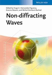
Figure 1.1 depicts (the real part of) an ordinary X-wave with and m.
Figure 1.1 Plot of the real part of the ordinary X-wave, evaluated for with a = 3 m.
Solutions (1.20) and, in particular, the pulse (1.23) have got an infinite field depth, and an infinite energy as well. Therefore, as was mentioned in the Bessel beam case, one should pass to truncated pulses, originating from a finite aperture. Afterward, our truncated pulses will keep their spatial shape (and their speed) along the depth of field
1.24
where, as before, is the aperture radius and the axicon angle (and is assumed to be much larger than the X-pulse spot).
At this point, it is worthwhile presenting Figure 1.2 and its caption.
Figure 1.2 All the X-waves (truncated or not) must have a leading cone in addition to the rear cone, such a leading cone having a role even for the peak stability [9]. Long ago, this was also predicted, in a sense, by (non-restricted [1, 13, 14]) special relativity: one should not forget, in fact, that all wave equations, and not only Maxwell's, have an intrinsic relativistic structure. By contrast, the fact that X-waves have a conical shape induced some authors to look for (untenable) links – let us now confine ourselves to electromagnetism – between them and the Cherenkov radiation, so as to to deny the existence of the leading cone: But X-shaped waves have nothing to do with Cherenkov, as it has been demonstrated thoroughly in Refs [34, 35, 96]. In practice, when wishing to produce concretely a finite conic NDW, truncated both in space and in time, one is supposed to have recourse in the simplest case to a dynamic antenna emitting a radiation cylindrically symmetric in space and symmetric in time [1].
For further X-type solutions, with less and less energy distributed along their “arms,” let us refer the reader to [12, 63] and references therein, as well as to [1]. For example, it was therein addressed the explicit construction of infinite families of generalizations of the classic X-shaped wave, with energy more and more concentrated around their vertex (see, e.g., Figure 1.9 in [1]). Elsewhere, techniques have been found for building up new series of non-diffracting superluminal solutions to the Maxwell equations suitable for arbitrary frequencies and bandwidths, and so on.
1.2 Eliminating Any Backward Components: Totally Forward NDW Pulses
As we mentioned, Equation 1.8, with its given by Equation 1.9, even if representing ideal solutions, is difficult to be used for obtaining analytical solutions with elimination of the “non-causal” components; a difficulty which becomes worse in the case of finite-energy NDWs. As promised, let us come back to these problems putting forth a method [63] for getting exact NDW solutions totally free of backward components.
Let us start with Equation 1.5 and Equation 1.6, which describe a general free-space solution (without evanescent waves) of the homogeneous wave equation, and consider in Equation 1.6 a spectrum of the type
1.25
where is the Kronecker delta function, the Heaviside function, and the Dirac delta function – quantity being an arbitrary function. Spectra of the type (1.25) restrict the solutions for the axially symmetric case, with only positive values to the angular frequencies and longitudinal wave numbers. With this, the solutions proposed by us get the integral form
1.26
that is, they result to be general superpositions of zero-order Bessel beams propagating in the positive -direction only. Therefore, any solution obtained from Equation 1.26, be it non-diffracting or not, are completely free from backward components.
At this point, we can introduce the unidirectional decomposition
1.27
with .
A decomposition of this type has been used until now in the context of paraxial approximation only [97, 98]; however, we are going to show that it can be much more effective, giving important results, in the context of exact solutions, and in situations that cannot be analyzed in the paraxial approach.
With Equation 1.27, we can write the integral solution 1.26 as
1.28
where , and where
1.29
are the new spectral parameters.
It should be stressed that superposition (1.28) is not restricted to NDWs: It is the choice of the spectrum that will determine the resulting NDWs.
1.2.1 Totally Forward Ideal Superluminal NDW Pulses
The most trivial NDW solutions are the X-type waves. We have seen that they are constructed by frequency superpositions of Bessel beams with the same phase velocity and until now constituted the only known ideal NDW pulses free ofbackward components. It is not necessary, therefore, to use the present method to obtain such X-type waves, as they can be obtained by using directly the integral representation in the parameters , that is, by using Equation 1.26. Even so, let us use our new approach to construct the ordinary X-wave.
Consider the spectral function given by
1.30
One can notice that the delta function in Equation 1.30 implies that , which is just the spectral characteristic of the X-type waves. In this way, the exponential function represents a frequency spectrum starting at , with an exponential decay and frequency bandwidth .
Using Equation 1.30 in Equation 1.28, we get
1.31
which is the well-known ordinary X wave.
Focus wave modes (FWMs) [12, 52, 54] are ideal non-diffracting pulses possessing spectra with a constraint of the type (with ), which links the angular frequency with the longitudinal wave number, and are known for their strong field concentrations.
Until now, however, all the known FWM solutions possessed backward spectral components, a fact that, as we know, forces one to consider large-frequency bandwidths to minimize their contribution. However, we are going to obtain solutions of this type free of backward components and able to possess also very narrow frequency bandwidths.
Let us choose a spectral function like
1.32
with a constant. This choice confines the spectral parameters of the Bessel beams to the straight line , as it is shown in Figure 1.3.
Figure 1.3 The Dirac delta function in Equation 1.32 confines the spectral parameters of the Bessel beams to the straight line , with .
Substituting Equation 1.32 in Equation 1.28, we have
1.33
which, on using identity in [99], results in
1.34
where is the ordinary X-wave given by Equation 1.31.
Equation 1.34 represents an ideal superluminal NDW of the type FWM, but free from backward components.
As we already said, the Bessel beams constituting this solution have their spectral parameters linked by the relation ; thus, by using Equation 1.32 and Equation 1.29, it is easy to see that the frequency spectrum of those Bessel beams starts at with an exponential decay , and so possesses the bandwidth . It is clear that and can assume any values, so that the resulting FWM, Equation 1.34, can range from a quasi-monochromatic to an ultrashort pulse. This is a great advantage w.r.t. the old FWM solutions.


