151,99 €
Mehr erfahren.
- Herausgeber: Wiley-VCH
- Kategorie: Wissenschaft und neue Technologien
- Sprache: Englisch
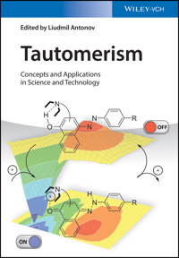
Reflecting the substantially increased interest in tautomerism, this book demonstrates the transformation of fundamental knowledge into novel concepts and the latest applications. Each chapter introduces the theoretical background, before reviewing and critically discussing the experimental techniques and corresponding applications. Special emphasis is placed on tautomerism under unusual conditions, such as in supramolecular solids and at surfaces, displaying the wide scope between basic research and timely applications.
Sie lesen das E-Book in den Legimi-Apps auf:
Seitenzahl: 746
Veröffentlichungsjahr: 2016
Ähnliche


Table of Contents
Cover
Related Titles
Title Page
Copyright
List of Contributors
Preface
References
Chapter 1: Tautomerism: A Historical Perspective
1.1 Thermodynamic Aspects
1.2 Kinetic Aspects
1.3 Conclusions
References
Chapter 2: “Triage” for Tautomers: The Choice between Experiment and Computation
2.1 Introduction (Original Text Written by Peter J. Taylor)
2.2
cis
-Amides
2.3 Tautomerism in Alicyclic Lactams: Six-Membered Rings
2.4 Tautomerism in Alicyclic Lactams: 2-Pyrrolidinone
2.5 Tautomerism in Other Five-Membered Ring Lactams
2.6 Tautomeric Ratios Requiring Computation: Alicyclic β-Diketones
2.7 Tautomeric Ratios Requiring Computation: “Maleic Hydrazide”
2.8 Tautomer Ratios Requiring Computation: 2-Oxo Derivatives of Pyrrole, Furan, and Thiazole
2.9 Tautomeric Ratios Requiring Computation: Compounds Containing Contiguous Carbonyl Groups
2.10 Tautomeric Ratios Requiring Computation: Compounds Containing Contiguous π-Donors
2.11 Compounds Equally Suited to Experiment or Computation: “Azapentalenes”
2.12 Phenomena Susceptible to Experiment or Computation: Lone Pair Effects
2.13 Conformational Effects on Aminoenone Stability: A Computational Approach
2.14 Overview (Original Text Written by Peter J. Taylor)
References
Chapter 3: Methods to Distinguish Tautomeric Cases from Static Ones
3.1 Introduction
3.2 The Liquid State
3.3 UV/VIS Spectroscopy
3.4 Infra Red Spectroscopy
3.5 Tautomerism in the Excited State
3.6 Near-Edge X-Ray
3.7 Energy-Dispersive X-Ray
3.8 Solid State
3.9 Single Molecule Tautomerization
3.10 Gas Phase
3.11 Theoretical Calculations
References
Chapter 4: Electron-Transfer-Induced Tautomerizations
4.1 Introduction
4.2 Methodology
4.3
O
-Alkyl Phenyl Ketones
4.4 Conclusions
Acknowledgments
References
Chapter 5: The Fault Line in Prototropic Tautomerism
5.1 Introduction: “
N
-Type” and “
C
-Type” Tautomerism
5.2 Tautomerism in Symmetrical Amidines
5.3 Tautomer Ratio in Asymmetric Heteroaromatic Amidines
5.4 Tautomer Ratio in the Imine–Enamine System: Substitution at Nitrogen
5.5 Tautomer Ratio in the Imine–Enamine System: Substitution at Carbon
5.6 The Resonance Contribution to Ketone and Amide Tautomerism
5.7 The Field-Resonance Balance in Vinylogous Heteroaromatic Amidines
5.8 Conclusions
References
Chapter 6: Theoretical Consideration of In-Solution Tautomeric Equilibria in Relation to Drug Design
6.1 Introduction
6.2 Methodology
6.3 Equilibration Mechanism
6.4 Relation to Drug Design
6.5 In-solution Equilibrium Calculations
6.6 Concluding Remarks
References
Chapter 7: Direct Observation and Control of Single-Molecule Tautomerization by Low-Temperature Scanning Tunneling Microscopy
7.1 Brief Introduction to STM
7.2 Direct Observation of Single-Molecule Tautomerization Using STM
7.3 Concluding Remarks
Acknowledgments
References
Chapter 8: Switching of the Nonlinear Optical Responses of Anil Derivatives: From Dilute Solutions to the Solid State
8.1 Introduction
8.2 Experimental and Theoretical Methods
8.3 Second-Order Nonlinear Optical Responses of Anils
8.4 Conclusions
Acknowledgments
References
Chapter 9: Tautomerism in Oxoporphyrinogens and Pyrazinacenes
9.1 Introduction
9.2 Tautomerism in Oxoporphyrinogen, OxP
9.3 Multichromic Acidity Indicator Involving Tautomerism
9.4 Polytautomerism in Oxocorrologen, OxC
9.5 Tautomerism in Linear Reduced Fused Oligo-1,4-pyrazines (Pyrazinacenes)
9.6 Conclusion
References
Chapter 10: Enolimine–Ketoenamine Tautomerism for Chemosensing
10.1 Introduction
10.2 Prototropic Enolimine–Ketoenamine Tautomerism
10.3 Ionochromic Enolimine–Ketoenamine Tautomeric Systems for Ions Sensing
10.4 Concluding Remarks
Acknowledgments
References
Chapter 11: Tautomerizable Azophenol Dyes: Cornerstones for Advanced Light-Responsive Materials
11.1 Azobenzene-Based Light-Sensitive Materials
11.2 Azophenols: Tautomerizable Photochromes with Fast Switching Speeds
11.3 Sub-Millisecond Thermally Isomerizing Azophenols for Optically Triggered Oscillating Materials
11.4 Fast-Responding Artificial Muscles with Azophenol-Based Liquid Single Crystal Elastomers
11.5 Conclusion
References
Chapter 12: Controlled Tautomerism: Is It Possible?
12.1 Introduction
12.2 Manipulation of Electronic Properties of the Substituents
12.3 Tautomeric Tweezers
12.4 Tautomeric Cavities
12.5 Proton Cranes
12.6 Rotary Switches
12.7 Concluding Remarks
Acknowledgments
References
Chapter 13: Supramolecular Control over Tautomerism in Organic Solids
13.1 Crystal Engineering and Tautomerism in Molecular Solids
13.2 Supramolecular Synthons
13.3 Solid-State Tautomerism, Proton Transfer, and Hydrogen Bonding
13.4 Supramolecular Stabilization of Metastable Tautomers
13.5 Identification of Tautomeric Properties and Connectivity Preferences
13.6 Synthetic Methods
13.7 Supramolecular Interactions in Other Tautomeric Solids
References
Chapter 14: Proton Tautomerism in Systems of Increasing Complexity: Examples from Organic Molecules to Enzymes
14.1 Introduction
14.2 Hydrogen Bond Geometries and Proton Transfer
14.3 Tautomerizations without Requiring Reorganization of the Environment
14.4 Tautomerizations Requiring Reorganization of the Environment
14.5 Conclusions
Acknowledgments
References
Index
End User License Agreement
Pages
xv
xvi
xvii
xviii
xix
xx
1
2
3
4
5
6
7
8
9
11
12
13
14
15
16
17
18
19
20
21
22
23
24
25
26
27
28
29
30
31
32
33
34
35
36
37
38
39
40
41
42
43
44
45
46
47
48
49
50
51
52
53
54
55
56
57
58
59
60
61
62
63
64
65
66
67
68
69
70
71
72
73
75
76
77
78
79
80
81
82
83
84
85
86
87
88
89
90
91
92
93
94
95
96
97
98
99
100
101
102
103
104
105
106
107
108
109
110
111
112
113
114
115
116
117
118
119
120
121
122
123
124
125
126
127
128
129
130
131
132
133
134
135
136
137
138
139
140
141
142
143
144
145
147
148
149
150
151
152
153
154
155
156
157
158
159
160
161
162
163
164
165
166
167
168
169
170
171
172
173
174
175
176
177
178
179
180
181
182
183
184
185
186
187
188
189
190
191
192
193
194
195
196
197
198
199
200
201
202
203
204
205
206
207
208
209
210
211
212
213
214
215
216
217
218
219
220
221
222
223
224
225
226
227
228
229
230
231
232
233
234
235
236
237
238
239
240
241
242
243
244
245
246
247
248
249
250
251
253
254
255
256
257
258
259
260
261
262
263
264
265
266
267
268
269
270
271
273
274
275
276
277
278
279
280
281
282
283
284
285
286
287
288
289
290
291
292
293
294
295
296
297
298
299
300
301
302
303
304
305
306
307
308
309
310
311
312
313
314
315
316
317
318
319
320
321
322
323
324
325
326
327
328
329
330
331
332
333
334
335
336
337
338
339
340
341
342
343
344
345
346
347
348
349
350
351
352
353
354
355
356
357
358
359
360
361
362
363
364
365
366
367
368
369
370
371
372
373
374
375
376
377
Guide
Cover
Table of Contents
Preface
Begin Reading
List of Illustrations
Chapter 1: Tautomerism: A Historical Perspective
Figure 1.1 Tautomeric equilibrium disturbed by a molecular modification.
Chapter 2: “Triage” for Tautomers: The Choice between Experiment and Computation
Figure 2.1 The relationship between
trans-
1a
and
cis
-
1b
amides and their iminols
2a
and
2b
.
Figure 2.2 Orbital interactions of iminoethers
3
and energy estimates for iminols
4
.
Figure 2.3 Tautomers of six-membered ring lactams, and related fixed forms.
Figure 2.4 Isodesmic treatment of
8
employing data from
5
to
9–18
.
Figure 2.5 Tautomeric possibilities in five-membered ring oxoheterocycles related to
8
.
Figure 2.6 Enolization in some β-diketones.
Figure 2.7 p
K
a
values for uracil
31
and the fixed forms
32
and
33
; estimates if bracketed.
Figure 2.8 Protonation scheme for “maleic hydrazide”
34
and model compounds
35–37
.
Figure 2.9 Tautomerism in
38
and
39
, Z = O, S, NH, and NMe.
Figure 2.10 Allylic tautomerism as quantified for various R
2
in Table 2.1.
Figure 2.11 Tautomerism in biacetyl
41
and cyclohexane-1,2-dione
42
.
Figure 2.12 α-Dicarbonyl compounds
43
and
44
, and orbital interactions in
45
.
Figure 2.13 Triazolones, and so on, which exist as the tautomer shown in aqueous solution.
Figure 2.14 Triazolones and oxadiazoles suggested for computational assessment.
Figure 2.15 Examples of azapentalene behavior [41] plus
59
, a partial rationale.
Figure 2.16 Diagrammatic representation of 2-aminoazole tautomerism.
Figure 2.17 2-Aminoazoles that provide
σ
I
and/or
K
M
at the point of attachment for NH
2
.
Figure 2.18 A sequence of azapentalenes designed to provide tautomer ratios.
Figure 2.19 p
K
a
and UV data in water for
74a
,
74b
, and their common cation
74h
.
Figure 2.20 Two examples of tautomerization from β-iminoketone to aminoenone.
Figure 2.21 The four planar conformations of simple aminoenones and their iminols.
Figure 2.22 Tautomerism in five-membered ring acylamidines.
Chapter 3: Methods to Distinguish Tautomeric Cases from Static Ones
Figure 3.1 Temperature variation of the CO chemical shift of β-thioxoketones.
3
R = Ph R
1
= CH
3
and
4
R = Ph R
1
= Ph (see Figure 3.2). H and D refer to the species with H or D at the OH/SH group.
Figure 3.2 Tautomeric equilibrium for β-thioxoketones.
Figure 3.3 Tautomeric forms of β-diketones.
Figure 3.4
1
H NMR spectrum of acetyl acetone.
1
Figure 3.5 XH chemical shifts plotted with the factor 1 parameter from a PCA analysis. Value 1 is probably an incorrect data. 2 and 3 illustrate temperature variations.
Figure 3.6 Tautomers of 1,2,3-triazole. To the left
T-2H
and to the right
T-1H
.
Figure 3.7 Schiff bases.
Figure 3.8 (a)
o
-Hydroxyazo-hydrazo tautomerism and (b,c) hydrazo forms.
Figure 3.9 Plot of calculated O…O distance versus
17
O chemical shifts. Open symbols are tautomeric compounds.
Figure 3.10 Structure of 1-propionyl-2-hydroxynaphthalene (
7
). The C=O group is twisted out of the ring plane.
Figure 3.11 Observed deuterium isotope effects on
13
C chemical shifts of β-diketones as a function of the mole fraction.
Figure 3.12 Equilibrium deuterium isotope effects on
13
C chemical shifts of β-diketones as a function of the mole fraction.
Figure 3.13 Tautomeric equilibrium of the enol form of 2-acetylcyclohexanone. Mole fraction,
x
.
Figure 3.14 Plot of deuterium isotope effects on
13
C chemical shifts for
o
-hydroxy Schiff bases.
Figure 3.15 Signs of deuterium isotope effects on
13
C chemical shifts for
o
-hydroxy Schiff bases.
Figure 3.16 Plot of factor 1 from PCA analysis versus the
13
C chemical shifts for C-2.
Figure 3.17
1
Δ
15
N(D) versus one-bond NH coupling constants.
Figure 3.18 Plot of
5
Δ
17
O(OD) versus
2
ΔC(OD) isotope effects.
Figure 3.19 Isotopic perturbation of equilibrium.
Figure 3.20
1
H and
2
H decoupled
13
C NMR spectrum of the statistical mixture of
3
,
3
-
d
1
, and
3
-
d
2
in CDCl
3
at −37.9 °C.
Figure 3.21 Explanation of observed isotope effects in the 2-phenylmalonaldehyde system deuterated at the aldehyde proton.
Figure 3.22
o
-Hydroxy acylaromatics.
Figure 3.23 Potential wells showing also zero point energy levels for H and D.
Figure 3.24 Plot of sum of secondary deuterium isotope effects on
13
C chemical shifts versus primary deuterium isotope effects.
Figure 3.25 Multiple equilibrium in citrinin.
Figure 3.26 Tautomeric structures of 3,6-dimethyl-1,8-dihydroxy-2-acetylnaphthalene.
Figure 3.27 Structures of 3,6-dimethyl-1,8-dihydroxy-2,7-diacetylnaphthalene.
Figure 3.28 Plot of
5
Δ
17
O(OD) versus primary deuterium isotope effects.
Figure 3.29 UV spectrum of (
E
)-4-chloro-2-(1-(methylimino)ethyl)-6-nitrophenol in CD
2
Cl
2
at variable temperature.
Figure 3.30 UV spectrum recorded in an NMR tube at 175 K in CD
2
Cl
2
. A2H is 4-nitrophenol and the acid is pivalic acid.
Figure 3.31 Keto-forms of
o
-hydroxy Schiff bases.
Figure 3.32 Excitation and tautomerism of porphycene.
Figure 3.33 Tautomerism of porphyrine.
Figure 3.34 Malonic acid enolization.
Figure 3.35 Tautomeric structures of
N
-(5-ethyl-1,3,4-thiadiazol-2-yl)-
p
-toluenesulfonamide.
Figure 3.36 Difference Fourier map in the mean plane of the H-bond chelate ring for compound (
E
)-1-(phenyldiazenyl)napthalen-2-ol at the temperatures of 100, 150, 200 K. Maps were computed after least-squares refinement carried out excluding the H-bond proton. Positive (continuous) and negative (dashed) contours drawn at 0.04 e Å
−3
intervals.
p
(N−H) refer to the mole fraction.
Figure 3.37 Change in dipole moments upon tautomerization of porphycene.
Figure 3.38 Panels (a–d) shows two dipoles in the plane but at different angles in the focal area of the azimuthally polarized doughnut mode (the direction of the light polarization is shown by the white arrows). Panels (e–h) showing the calculated excitation patterns.
Figure 3.39 Spatial pattern of fluorescence from two single molecules of porphycene embedded in PMMA film. Experiments at top, simulations below.
Figure 3.40 Calculated nuclear shielding surface for the C-α carbon of an
o
-substituted Schiff base. The NH bond length is varied.
Figure 3.41 (a) Plot of experimental chemical shifts versus calculated nuclear shieldings for hydrazo form I (see Figure 3.43). (b) Plot of experimental chemical shifts versus calculated nuclear shieldings for hydrazo form IV (see Figure 3.43).
Figure 3.43 Likely structures.
Figure 3.42 Tautomeric forms suggested in Ref. [15]. R= Phe and R'= methyl.
Figure 3.44 Compounds used in the calculation of
1
J
(
15
N,H).
Figure 3.45 Experimental IR spectrum (called before irradiation) together with calculated spectra.
Chapter 4: Electron-Transfer-Induced Tautomerizations
Scheme 4.1
Figure 4.1 Relative energies of the keto and enol form of
o
-methylbenzaldehyde and their radical cations, from B3LYP/6-31G* calculations.
Figure 4.2 Spectra obtained on ionization of benzophenone (a) and
o-
methylbenzophenone (b) in a solid Ar matrix at 10 K. (c) Spectrum obtained on photolysis of spectrum (b) at 500 nm. (d) Spectrum obtained on pulse radiolysis of
o-
methylbenzophenone [11].
Figure 4.3 Peaks in the O−H stretching region of the enol radical cation
2
•+
(R = H, R′ = Ph), and their change upon irradiation at 500 nm (cf. Figure 4.2) [11].
Scheme 4.2
Figure 4.4 UV/Vis and IR spectra of the enol radical cation of
o
-methylacetophenone, generated from
o
-methylacetophenone (bottom) and from methylbenzocyclobutenol (top, cf. Scheme 4.1) [12]. The dashed lines show the spectral changes upon photolysis at 700 nm, which are due to conformational changes.
Figure 4.5 (a) Spectra of the enol radical cation of
o
-methylacetophenone and its deuterated derivative obtained by pulse radiolysis in solid butyl chloride; (b) workup of the data according to classical first-order kinetics; and (c) workup of the data according to dispersive kinetics [12].
Figure 4.6 Arrhenius plots for the enolization of the radical cation of
o
-methylacetophenone and its deuterated derivative. Solid lines are from the Bell model.
Scheme 4.3
Figure 4.7 UV-Vis spectra obtained on ionization and subsequent photolyzes of 7-methyl (
7
) and 4,7-dimethyl-1-indanone (
6
) and their deuterated derivatives. Black vertical bars indicate results of CASPT2 excited state calculations [17].
Figure 4.8 Changes in the IR spectra of ionized dimethylindanone on photolysis [17].
Figure 4.9 Comparison of photoenolization of enones (a) and enolization of the corresponding radical cations (b) in terms of their electronic structure.
Figure 4.10 Potential energy diagram for the enolization of
6
(R = Me, open bars, dashed lines) and
7
(R = H, full bars, solid lines).
Scheme 4.4
Scheme 4.5
Scheme 4.6
Figure 4.11 UV-Vis and IR spectra obtained in Ar matrices after ionization of NADH analogs. Dashed line: spectrum obtained after photolysis at 510 nm or overnight standing at 12 K [20]. Black vertical bars: predictions from excited state calculations for
8 K
(by CASPT2) and for
10 E
(by TD-DFT).
Scheme 4.7
Chapter 5: The Fault Line in Prototropic Tautomerism
Figure 5.1 The distinction between “N-type” and “C-type” tautomerism [1].
Figure 5.2 Protonation of symmetrical guanidines.
Figure 5.3 Compounds relevant to the estimation of amidine/guanidine tautomer ratios.
Figure 5.4 The sketch of the relation between p
K
a
and
σ
I
for the tautomers of symmetrical amidines.
Figure 5.5 p
K
a
values of some substituted guanidines.
Figure 5.6 Imines and enamines from which log
K
M
for R = alkyl and Ph may be deduced.
Figure 5.7 The three-way tautomerism of azo- (
28
) and nitroso- (
29
) compounds.
Figure 5.8 Tautomerism in imines
14
for which R is a π-acceptor.
Figure 5.9 Fixed (
35
,
36
) and mobile (
34
) tautomers of some 4-amino-2-pyrimidones.
Figure 5.10 Tautomerism in some anydro-bases
37
.
Figure 5.11 Influence of substituents on ketone (
38)
and amide (
39, 40
) tautomerism.
Figure 5.12 Tautomerism in heteroaromatic amidines
12
and their vinylogous
41
.
Chapter 6: Theoretical Consideration of In-Solution Tautomeric Equilibria in Relation to Drug Design
Figure 6.1 Double proton-relay in the dimers; 2-hydroxy pyridine (
1
) to 2-pyridone (
2
) and 1
H
,3
X
-pyrazole (
3
) to 2
H
,3
X
-pyrazole (
4
).
Figure 6.2 Three largely different warfarin tautomers out of eight [32], as discussed above.
Figure 6.3 Protonation at N
1
(
5
) and N
4
(
6
) of the piperazine (P) ring.
Figure 6.4 Tautomers of 5-hydroxyisoxazole and its methyl and dimethyl derivatives (R
1
, R
2
= all combinations of H and CH
3
) (
7–9
); tautomeric equilibria for methylphosphino- (R
3
= CH
3
) and phenylphosphino (R
3
= phenyl)-substituted cyclic imidazoline, oxazoline, and thiazoline systems, X = NH, O, S, respectively (
10
phosphino,
11
phosphinidene).
Figure 6.5 Tautomeric transformations for asymmetrically substituted five-member heterocycles. Imidazole, 1
H
,4
X
to 3
H
,4
X
(
12
,
13
); tetrazole, 2
H
,5
X
to1
H
,5
X
, (
14, 15
); 1,2,3-triazole, 1
H
,4
X
to 2
H
,4
X
to 3
H
,4
X
, (
16–18
); and 1,2,4 triazole, 1
H
,3
X
to 2
H
,3
X
to 4
H
,3
X
, (
19–21
).
Figure 6.6 Direct double proton-relay in the natural guanine–cytosine pair
G
⋯
C
resulting in the formation of a rare complex
(G
⋯
C)′
.
Figure 6.7 Neurotransmitters in their neutral forms. Dopamine (
22
); norepinephrine (
23
); epinephrine (
24
); tyramine (
25
); and serotonin (
26
). Zwitterions are formed when a hydroxyl proton moves to the amine nitrogen of the molecule.
Figure 6.8 Selected tautomers/conformers for malondialdehyde, diketo (
27
), all
trans
enol–keto (
28
), and for acetylacetone, s-
cis
enol–keto (
29
), diketo (
30
).
Chapter 7: Direct Observation and Control of Single-Molecule Tautomerization by Low-Temperature Scanning Tunneling Microscopy
Figure 7.1 STM working principle. (a) Schematics of a typical STM configuration. A metal tip mounted on piezo positioners (
x
,
y
, and
z
direction) is scanned over a conductive surface. The displacement (Δ
z
) of the tip is controlled by a feedback loop while keeping the tunneling current constant. An STM image is constructed by raster scanning over the surface. Note that both bias polarities can be used, resulting in an electric current flow toward the surface or toward the tip. (b) Schematics of a simple metal (tip)–vacuum–metal (surface) junction. (c) Hybridization of molecular orbitals upon adsorption on a surface.
Figure 7.2 Direct observation of molecular states (pentacene on a Au(111) surface). (a) STS spectrum of a pentacene molecule (the chemical structure is shown in the inset). (b) STM (topography) images (left), d
I
/d
V
mapping, and simulated image of molecular orbitals of a pentacene molecule on a Au(111) surface.
Figure 7.3 Schematic model of the inelastic electron tunneling process. An electron can tunnel inelastically (denoted as e
−
(inel)) in addition to the elastic channel (denoted as e
−
(el)) when the electron energy
eV
is larger than a specific vibration energy (
ℏ
Ω) within a molecule on a surface. In the inelastic process, the electron loses the energy and leaves vibrational quanta (here
m
+ 1 ←
m
is assumed with
m
being the vibrational quantum number) in the molecule.
Figure 7.4 Single naphthalocyanine molecule adsorbed on a two monolayer NaCl film on Cu(111). (a)
I–V
(black curve) and STS (d
I
/d
V
, gray curve) spectra measured for a single naphthalocyanine molecule. The inset shows a schematic illustration of the system. (b) STM images (top) at the bias voltage corresponding to the HOMO (left), gap (center), and LUMO (right). The simulated molecular orbitals and chemical structure are presented at the bottom. The position of the inner H atoms in the cavity determines the axis of the twofold symmetry in the LUMO.
Figure 7.5 Tautomerization of a single phthalocyanine molecule on a two monolayer NaCl film on Cu(111). (a) STM images of a single molecule before and after tautomerization (
V
= 0.7 V,
I
t
= 2 pA). The black dot in the left image indicates the position of the STM tip during a voltage pulse to induce the tautomerization. (b) Ball-and-stick model of the inner cavity. (c) Voltage dependence of the tautomerization rate.
Figure 7.6 Tautomerization of a single TPP molecule on a Ag(111) surface. (a) Pseudo-three-dimensional STM image of a single TPP molecule (b) Model of a TPP molecule on the surface. (c) STM images before and after tautomerization (
V
s
= −0.2 V,
I
t
= 0.1 nA), leading to two different tautomers (α- and κ-TPP). (d) Chemical structures corresponding to the STM images above (in (c)).
Figure 7.7 Four-state tautomerization of a singly dehydrogenated TPP molecule on Ag(111). The pyrrole ring with the H atom is observed as a protrusion in the STM images (as indicated by arrows).
Figure 7.8 Chemical structure and schematic of the inner cavity geometry of (a) porphycene and (b) porphine.
Figure 7.9 (a,b) Constant-current STM images of a single porphycene molecule adsorbed on Cu(110) (size: 1.49 × 1.42 nm
2
, gap conditions:
I
t
= 10 nA and
V
= 100 mV). The gray scale represents the apparent (topographic) height of the STM (i.e., the vertical displacement of the STM tip), and the zero point corresponds to the surface level. The white grid lines correspond to the surface lattice of Cu(110) underneath the molecule (the lattice constants are
a
0
= 2.55 Å and
b
0
= 3.61 Å). A molecule can be switched between two orientations through thermal- or STM-induced excitation. (c) Chemical structures of a porphycene molecule with the
cis
tautomer state. The switching between the two orientations in (a,b) corresponds to a
cis–cis
tautomerization.
Figure 7.10 Different tautomers of porphycene on Cu(110) as calculated by DFT:
trans
(a–c),
cis
-1 (d–f), and
cis
-2 (g–i). Chemical structures (a,d,g), optimized structures (b,e,h) (with the relative total energies indicated), and simulated STM images (c,f,i).
Figure 7.21 Tautomerization within porphycene row on Cu(110) at 5 K (Reproduced from Kumagai
et al.
[31]. Copyright (2014), with permission of Nature Publishing.). (a) STM image of a porphycene dimer (
V
t
= 100 mV and
I
t
= 20 nA, image size: 1.79 × 2.89 nm
2
; the grid represents the Cu(110) surface lattice). (b) Schematic of a porphycene dimer. (c–e) STM images of a trimer (1.47 × 4.33 nm
2
), tetramer (1.47 × 5.70 nm
2
), and pentamer (1.47 × 7.10 nm
2
) adjacent to an O row that does not influence tautomerization properties (supporting information in Ref. [31]). The images were acquired at
V
t
= 300 mV and
I
t
= 1 nA to induce continuous switching. (f–i) STM images (
V
t
= 100 mV and
I
t
= 1 nA) of one and the same trimer in various orientations of the termini molecules with (j) corresponding current histograms acquired at
V
t
= 300 mV. The tip position during the measurement is fixed at the location indicated by markers in (f–i) with the gap conditions of
V
t
= 100 mV and
I
t
= 10 pA.
Figure 7.11 (a–c) STM images of a single porphycene molecule on Cu(110) at different temperatures (as indicated). The fuzzy appearance results from switching between two orientations (
cis–cis
tautomerization). (d) Tunneling current dependence of the tautomerization rate measured at different temperature and bias voltages: at 77 K and
V
t
= 50 mV (open squares), and at 5 K and
V
t
= 200 mV (open circles). (e) Arrhenius plot for thermally activated tautomerization.
Figure 7.12 STM-induced
cis–cis
tautomerization of a porphycene molecule on Cu(110) at 5 K (Reproduced from Kumagai
et al.
[30]. Copyright (2013), with permission of Nature Publishing.). (a–h) Voltage-dependent STM images of a single porphycene molecule (the bias voltage is indicated;
I
t
= 5 nA; image size: 2 × 2 nm
2
; scanning time of approximately 9 s per image). (i) Current trace during a voltage pulse of 300 mV while the tip was fixed at the position indicated by the black star in (a) with gap conditions of
V
t
= 100 mV and
I
t
= 10 pA. (j) Current histogram obtained from the current trace in (i). (k,l) Schematics of “high” and “low” states.


