101 Most Popular Excel Formulas E-Book

Bryan Hong

• Herausgeber: MyExcelOnline
• Kategorie: Wissenschaft und neue Technologien
• Sprache: Englisch

Veröffentlichungsjahr: 2019

Beschreibung

Learn the Most Popular Excel Formulas Ever: VLOOKUP, IF, SUMIF, INDEX/MATCH, COUNT, SUMPRODUCT plus Many More!

With this book, you’ll learn to apply the must know Excel Formulas & Functions to make your data analysis & reporting easier and will save time in the process.

With this book you get the following:

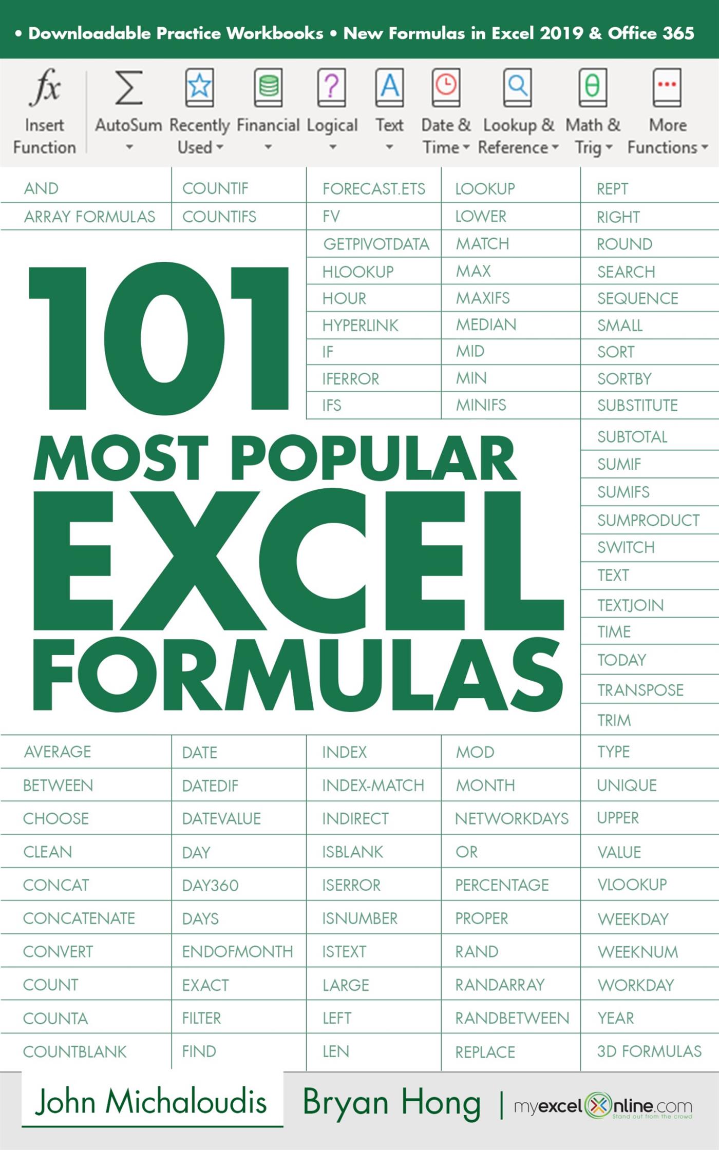
✔ 101 Ready Made Formulas Covering: LOOKUP, LOGICAL, MATH, STATISTICAL, TEXT, DATE, TIME & INFORMATION 
✔ Easy to Read Step by Step Guide with Color Screenshots
✔ Downloadable Practice Workbooks for each Formula with Solutions
✔ Interactive & Searchable E-Book to find any Formula with ease
✔ New Excel Formulas For Excel 2019 & Office 365

This book is a MUST-HAVE for Beginner to Intermediate Excel users who want to learn Excel Formulas FAST & stand out from the crowd!

Leseprobe

COPYRIGHT

Copyright © 2020 by MyExcelOnline.com – Version 1.2020

All rights reserved. This publication is protected by copyright, and permission must be obtained from the publisher prior to any prohibited reproduction, storage in a retrieval system, or transmission in any form or by any means, electronic, email, mechanical, photocopying, recording or likewise.

SPECIAL SALES

For more information about buying this eBook in bulk quantities, or for special sales opportunities (which may include custom cover designs, and content particular to your business or training goals), please send us an email to [email protected]

MYEXCELONLINE ACADEMY COURSE

We are offering you access to our online Excel membership course – The MyExcelOnline Academy – for only $1 for the first 30 days!

Click on this $1 Trial link to get access to this special reader offer!

CONNECT WITH US

Website, blog & podcast: https://www.myexcelonline.com/

Download Our App: Android or iPhone

Email: [email protected]

AUTHOR BIOGRAPHY

John Michaloudis is the founder of MyExcelOnline.com. John is currently living in the North of Spain, married and have two beautiful kids.John holds a bachelor’s degree in Commerce (Major in Accounting) and speak English/Australian, Greek and Spanish.

Bryan Hong is a contributor of MyExcelOnline.com. He is currently living in the Philippines and is married to his wonderful wife Esther.Bryan is also a Microsoft Certified Systems Engineer with over 10 years of IT and teaching experience!

HOW TO USE THIS E-BOOK

Formulas are one of the most powerful features in Excel and learning how & when to use them will make you into an Excel superstar! There are 483 Functions at the time of publishing this eBook but you only need to know several of these to become efficient at Excel!

To get the most value out of this eBook, we recommend that you download the workbook that pertains to each Function and practice entering the Function in a cell. Then follow our easy to use step by step guide. Make mistakes! That is fine. You may not get it the first time around (we certainly didn’t) but when you finally do, you will be a step closer to Excel stardom!

For the download link that has all of the workbooks covered in this eBook, please go to the last page.

The Table of Contents is interactive & will take you to a Function within this eBook!

Table of Contents

COPYRIGHT

SPECIAL SALES

MYEXCELONLINE ACADEMY COURSE

CONNECT WITH US

AUTHOR BIOGRAPHY

HOW TO USE THIS E-BOOK

Table of Contents

Formulas VS Functions

FORMULA TIPS

The Function Wizard

F9 to Evaluate a Formula

Named Ranges

Absolute & Relative References

Evaluate Formulas Step By Step

Highlight All Excel Formula Cells

How to Convert Formulas to Values

How to Show & Hide Formulas in Excel

Jump to a Cell Reference in a Formula

LOOKUP FUNCTIONS

ADDRESS

CHOOSE

HLOOKUP

HYPERLINK

INDEX

INDEX-MATCH

INDIRECT

LOOKUP

MATCH

VLOOKUP

LOGICAL FUNCTIONS

AND

IF

IFERROR

OR

MATH FUNCTIONS

COUNT

COUNTA

COUNTBLANK

COUNTIF

COUNTIFS

MOD

PERCENTAGE

RAND

RANDBETWEEN

ROUND

SUBTOTAL

SUMIF

SUMIFS

SUMPRODUCT

STATISTICAL FUNCTIONS

AVERAGE

LARGE

MAX

MEDIAN

MIN

SMALL

TEXT FUNCTIONS

CLEAN

CONCATENATE

EXACT

FIND

LEFT

LEN

LOWER

MID

PROPER

REPLACE

RIGHT

SEARCH

SUBSTITUTE

TRIM

UPPER

VALUE

DATE & TIME FUNCTIONS

DATE

DATEDIF

DATEVALUE

DAY

DAY360

DAYS

ENDOFMONTH

HOUR

MONTH

NETWORKDAYS

TODAY

WEEKDAY

WEEKNUM

WORKDAY

YEAR

INFORMATION FUNCTIONS

ISBLANK

ISERROR

ISNUMBER

ISTEXT

TYPE

OTHER FUNCTIONS

FV – Compound Interest

FV – Monthly Investment

EXCEL 2019

CONCAT

IFS

MAXIFS

MINIFS

SWITCH

TEXTJOIN

OFFICE 365

FILTER

RANDARRAY

SEQUENCE

SORT

SORTBY

UNIQUE

ADVANCED FORMULAS

3D Formulas

ARRAY Formulas

BETWEEN

Extract First Name from Full Name

Extract Last Name - REPLACE Function

GETPIVOTDATA

IF Combined With The AND Function

INDEX-MATCH 2 Criteria with Validation

Match Two Lists With MATCH Function

Named Ranges with VLOOKUP Function

REPT

SUMPRODUCT: Sum Multiple Criteria

SUMPRODUCT: Sum the Top 3 Sales

TIME – Get Elapsed Time

TRANSPOSE

VLOOKUP Approximate Match

VLOOKUP with a Drop Down List

VLOOKUP Multiple Columns

VLOOKUP with Multiple Criteria

MYEXCELONLINE ACADEMY COURSE

Formulas VS Functions

You most probably have heard the words Formulas & Functions both being used in Excel. What is the difference between them?

A Formula is an expression which calculates the value of a cell. A Function is a predefined formula that is made available for you to use in Excel:

In this book, we use both terms (function and formula) interchangeably.

Here are several operators that you can use in a Formula:

FORMULA TIPS

The Function Wizard

What does it do?

If you are unsure on which formula to use in Excel, Excel has you covered! You can use the Insert Function Wizard of Excel to find one for your purpose.

STEP 1:Ensure you have a cell selected and click the Insert Function button depicted as fx:

STEP 2:Inside this window, you can try to search for the function:

Or filter by category:

STEP 3:Once you have selected the function you want, click OK.

STEP 4:Fill out the arguments of your selected function. Click OK.

Your Excel Formula is now ready!

F9 to Evaluate a Formula

What does it do?

Sometimes we need to create complicated formulas, and when that happens it is easy to make mistakes. It becomes hard finding what caused the issue! The fun part is it is easy to evaluate parts of your Formula in Excel by using pressing the F9 Key!

Our example checks if the date is in the Month of January and has sales greater than 1000. It uses the AND Function and we want to understand why it evaluated to FALSE.

Exercise Workbook:

DOWNLOAD EXCEL WORKBOOK

STEP 1: Double click or press F2 on the cell that has the formula

STEP 2: Select the part of the formula that you want to evaluate first. Let us check the first part: MONTH(C9)=1

Press F9 to evaluate this part. It evaluates to FALSE because the month in cell C9 is February and not January or 1

STEP 3: Let us evaluate the second part of the formula. Select the other part: D9 >1000

Press F9 to evaluate this part. It evaluates to TRUE because D9 is greater than 1000.

Press ESC to exit the formula editor without making changes.

Now it makes sense why our formula here gave us a value of FALSE!

Named Ranges

What does it do?

A named range in Excel is a cell or range of cells that has a more descriptive name. It goes a long way in using named ranges, because it allows you to create cleaner and easier to understand formulas in Excel!

Our example gets the maximum value with the MAX Function. Let us improve this function by replacing the range of cells with a named range.

Exercise Workbook:

DOWNLOAD EXCEL WORKBOOK

STEP 1: Select the cells that you want to give a named range to.

STEP 2: Go to Formulas > Defined Names > Define Name

STEP 3: Give it a meaningful name (it cannot have spaces) and click OK.

STEP 4: Let us now update our formula to use our named range!

Our formula looks way better now and is still working as expected!

Absolute & Relative References

What does it do?

When creating formulas, it is very important to understand cell references. Let us go over the differences between absolute and relative references.

It will affect how your cell references will appear when you copy an Excel formula from one cell to another.

Exercise Workbooks:

DOWNLOAD EXCEL WORKBOOK (Relative Reference exercise)

DOWNLOAD EXCEL WORKBOOK (Absolute Reference exercise)

Excel uses relative references by default. A relative reference is useful if you want to use the same pattern across different cells.

For example, we have here a formula that gets the YEAR from cell C9.

STEP 1: If we drag this formula all the way down for it to be copied to other cells:

Notice that the cell references have changed as well:

You could tell that Excel was smart enough to get the year of the left cell which contains the date without us even making a single change.

For absolute references, the reference to a cell is always fixed even if we copy our formula to another cell.

We have this example that uses a NETWORKDAYS function. A NETWORKDAYS Function needs a list of holidays to count the correct number of working days.

Since we want to use the NETWORKDAYS function multiple times, it would make sense to have a single list of holidays for it to use. This is where the absolute reference comes in handy.

An absolute reference contains a $ symbol in front of the column letter and the row number. You can see in our example that it has $A$9:$A$11 pertaining to our Holiday Table. Notice that there are relative cell references in the formula as well (e.g. C9 and D9).

STEP 2: The magic happens when we drag our formula downwards.

If we look at the other formulas, the Holiday table is exactly the same and has not changed ($A$9:$A$11). While the relative cell references have changed (e.g. C10 and D10, C11 and D11, C12 and D12).

Knowing when to use absolute or relative cell reference will be a crucial skill. It will make your work a lot easier when copying the same formula across multiple cells.

TIP: You can press the F4 key to enter an absolute reference.

Pressing the F4 key multiple times, will change the absolute/relative reference combination to a mixed reference.

Give it a try!

Evaluate Formulas Step By Step

What does it do?

This is one of the coolest tricks I have seen in Excel, as there are countless times where I had a hard time understand formulas. Especially long and complex ones!

Excel provides the way to evaluate your formula, and break it down step by step so that you can understand it!

Let us take the formulas I've created below in the IS THE VALUE IN BETWEEN column. We will see how this formula is resolved in a series of steps:

Exercise Workbook:

DOWNLOAD EXCEL WORKBOOK

STEP 1:You can see our formula uses both the If formula and the Median formula. 

The goal of this formula is to evaluate if a value (VALUE TO BE EVALUATED) is in between the range (START OF RANGE to VALUE TO BE EVALUATED)

For example: Is 50 the median of the range 20; 60; 50?

=IF(C7=MEDIAN(A7:C7), "Yes", "No")

To start understanding our formula, highlight the formula, then go to Formulas > Evaluate Formula:

STEP 2: Our formula is now shown on screen, and the part that is underlined is the one to be evaluated first.  Click Evaluate.

STEP 3:C7 has been evaluated to 50.  Click Evaluate.

STEP 4:  The median of the values from A7 to C7 (20, 60, 50) is evaluated as 50.  Click Evaluate.

STEP 5:  Is 50 equal to 50?

Excel has evaluated it to TRUE.  Click Evaluate.

STEP 6:  Since the If formula received a TRUE, Excel evaluated it as a Yes end result. We have seen how the formula gave us the result in a few easy steps!

Highlight All Excel Formula Cells

What does it do?

Whenever you are auditing an Excel worksheet and need to know where all the formulas are located, a great way is to highlight the formula cells in a distinctive color. 

Exercise Workbook:

DOWNLOAD EXCEL WORKBOOK

STEP 1: Select all the cells in your Excel worksheet by clicking on the top left hand corner of your worksheet.

STEP 2: Press the CTRL+G shortcut which will open up the Go To dialogue box and select the Specialbutton.

STEP 3: Select the Formularadio button and press OK.

STEP 4: This will highlight all the formulas in your Excel worksheet and you can use the Fill Color to color in the formula cells.

And now all your cells containing formulas are now highlighted!

How to Convert Formulas to Values

What does it do?

Have you ever had a scenario where you write a formula and just want to show the value output only and get rid of the formula?

Here is an example of a formula:

Well I do not need the formula, bit I do want the last names only....hard copied!

Fortunately, I have discovered two ways that you can achieve this...

Exercise Workbook:

DOWNLOAD EXCEL WORKBOOK

STEP 1:Select the area that contains the formulas.

Click CTRL+C

On the column that you want to place the values on, right-click and select Paste Values: 

You can see that the actual values are now stored in that column!

STEP 2: Here's an alternative way.  Select the area that contains the formulas.

Right-click and hold on the right border.

Drag the border, whilst holding down the right-click on your mouse, to the area you want the values to be placed in.

Select Copy Here as Values Only.

You now have the actual values hardcoded!

How to Show & Hide Formulas in Excel

What does it do?

When I have a sheet full of Excel formulas, sometimes I want to quickly check how each formula looks like.  This is great for spreadsheet auditing.

It is very easy to do so in Excel!

Here is our sample worksheet with formulas:

Exercise Workbook:

DOWNLOAD EXCEL WORKBOOK

STEP 1:Press on your keyboard the following keys: Ctrl + `

The (`) key is usually located on the upper left part of your keyboard. This will show all your Excel formulas in your worksheet!

Press the Ctrl + ` combination again to hide the formulas.

STEP 2: If you prefer to set this via Excel Options, another way is to go to File > Options

STEP 3: Go to Advanced> Display Options for this Worksheet > Show formulas in cells instead of their calculated fields

Ensure this is checked.

The formulas are all shown now too!  You can uncheck it to hide the formulas again.