139,99 €
Mehr erfahren.
- Herausgeber: John Wiley & Sons
- Kategorie: Wissenschaft und neue Technologien
- Sprache: Englisch
Most physical problems can be written in the form of mathematical equations (differential, integral, etc.). Mathematicians have always sought to find analytical solutions to the equations encountered in the different sciences of the engineer (mechanics, physics, biology, etc.). These equations are sometimes complicated and much effort is required to simplify them. In the middle of the 20th century, the arrival of the first computers gave birth to new methods of resolution that will be described by numerical methods. They allow solving numerically as precisely as possible the equations encountered (resulting from the modeling of course) and to approach the solution of the problems posed. The approximate solution is usually computed on a computer by means of a suitable algorithm. The objective of this book is to introduce and study the basic numerical methods and those advanced to be able to do scientific computation. The latter refers to the implementation of approaches adapted to the treatment of a scientific problem arising from physics (meteorology, pollution, etc.) or engineering (structural mechanics, fluid mechanics, signal processing, etc.) .
Sie lesen das E-Book in den Legimi-Apps auf:
Seitenzahl: 195
Veröffentlichungsjahr: 2018
Ähnliche
Table of Contents
Cover
Title
Copyright
Preface
PART 1: Introduction
1 Review of Linear Algebra
1.1. Vector spaces
1.2. Linear mappings
1.3. Matrices
1.4. Determinants
1.5. Scalar product
1.6. Vector norm
1.7. Matrix eigenvectors and eigenvalues
1.8. Using
Matlab
2 Numerical Precision
2.1. Introduction
2.2. Machine representations of numbers
2.3. Integers
2.4. Real numbers
2.5. Representation errors
2.6. Determining the best algorithm
2.7. Using
Matlab
PART 2: Approximating Functions
3 Polynomial Interpolation
3.1. Introduction
3.2. Interpolation problems
3.3. Polynomial interpolation techniques
3.4. Interpolation with the Lagrange basis
3.5. Interpolation with the Newton basis
3.6. Interpolation using spline functions
3.7. Using
Matlab
4 Numerical Differentiation
4.1. First-order numerical derivatives and the truncation error
4.2. Higher-order numerical derivatives
4.3. Numerical derivatives and interpolation
4.4. Studying the differentiation error
4.5. Richardson extrapolation
4.6. Application to the heat equation
4.7. Using
Matlab
5 Numerical Integration
5.1. Introduction
5.2. Rectangle method
5.3. Trapezoidal rule
5.4. Simpson’s rule
5.5. Hermite’s rule
5.6. Newton–Côtes rules
5.7. Gauss–Legendre method
5.8. Using
Matlab
PART 3: Solving Linear Systems
6 Matrix Norm and Conditioning
6.1. Introduction
6.2. Matrix norm
6.3. Condition number of a matrix
6.4. Preconditioning
6.5. Using
Matlab
7 Direct Methods
7.1. Introduction
7.2. Method of determinants or Cramer’s method
7.3. Systems with upper triangular matrices
7.4. Gaussian method
7.5. Gauss–Jordan method
7.6. LU decomposition
7.7. Thomas algorithm
7.8. Cholesky decomposition
7.9. Using
Matlab
8 Iterative Methods
8.1. Introduction
8.2. Classical iterative techniques
8.3. Convergence of iterative methods
8.4. Conjugate gradient method
8.5. Using
Matlab
9 Numerical Methods for Computing Eigenvalues and Eigenvectors
9.1. Introduction
9.2. Computing det (
A − λI
) directly
9.3. Krylov methods
9.4. LeVerrier method
9.5. Jacobi method
9.6. Power iteration method
9.7. Inverse power method
9.8. Givens–Householder method
9.9. Using
Matlab
10 Least-squares Approximation
10.1. Introduction
10.2. Analytic formulation
10.3. Algebraic formulation
10.4. Numerically solving linear equations by QR factorization
10.5. Applications
10.6. Using
Matlab
PART 4: Appendices
Appendix 1: Introduction to Matlab
A1.1. Introduction
A1.2. Starting up
Matlab
A1.3. Mathematical functions
A1.4. Operators and programming with
Matlab
A1.5. Writing a
Matlab
script
A1.6. Generating figures with
Matlab
Appendix 2: Introduction to Optimization
A2.1. Introduction
A2.2. Standard results on functions from ℝ
n
to ℝ
A2.3. Optimization without constraints
Bibliography
Index
End User License Agreement
List of Tables
3 Polynomial Interpolation
Table 3.1. Divided differences for Hermite interpolation
8 Iterative Methods
Table 8.1. Results of each iteration of the Jacobi method
Table 8.2. Results of each iteration of the Gauss–Seidel algorithm
Table 8.3. Results of the first seven iterations of the Gauss–Seidel method
Table 8.4. Results of the first seven iterations of the relaxation method
List of Illustrations
3 Polynomial Interpolation
Figure 3.1. Three examples of Lagrange functions
Figure 3.2. The function exp x and its interpolant p(x)
Figure 3.3. Interpolation error relative to the function exp x
Figure 3.4. Cubic spline
Figure 3.5. Newton interpolation
Figure 3.6. Interpolation of sin x between 0 and 3π
Figure 3.7. Interpolation of sin x between 0 and 10
Figure 3.8. Interpolation of cos x between 0 and 10
5 Numerical Integration
Figure 5.1. Illustration of the rectangle method
Figure 5.2. Illustration of the trapezoidal rule
Figure 5.3. Illustration of Simpson’s rule
6 Matrix Norm and Conditioning
Figure 6.1. Geometric illustration of the matrix norm
9 Numerical Methods for Computing Eigenvalues and Eigenvectors
Figure 9.1. Three-story building
Figure 9.2. Discretization of the beam
Figure 9.3. The first modes calculated by the script
Appendix 1: Introduction to Matlab
Figure A1.1. Matlab window
Appendix 2: Introduction to Optimization
Figure A2.1. Illustration of global and local minima
Guide
Cover
Table of Contents
Begin Reading
Pages
C1
iii
iv
v
xi
xii
1
3
4
5
6
7
8
9
10
11
12
13
14
15
16
17
18
19
21
22
23
24
25
26
27
28
29
30
31
32
33
35
37
38
39
40
41
42
43
44
45
46
47
48
49
50
51
52
53
54
55
56
57
58
59
60
61
62
63
64
65
67
68
69
70
71
72
73
74
75
76
77
78
79
80
81
83
84
85
86
87
88
89
90
91
92
93
94
95
96
97
98
99
100
101
102
103
104
105
107
109
110
111
112
113
114
115
116
117
118
119
120
121
123
124
125
126
127
128
129
130
131
132
133
134
135
136
137
138
139
140
141
142
143
144
145
147
148
149
150
151
152
153
154
155
156
157
158
159
160
161
163
164
165
166
167
168
169
170
171
172
173
174
175
176
177
178
179
180
181
182
183
185
186
187
188
189
190
191
192
193
194
195
196
197
198
199
201
202
203
204
205
206
207
208
209
210
211
212
213
215
217
218
G1
G2
G3
G4
G5
G6
G7
e1
Mathematical and Mechanical Engineering Set
coordinated by
Abdelkhalak El Hami
Volume 6
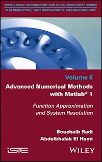
Advanced Numerical Methods with Matlab® 1
Function Approximation and System Resolution
Bouchaib Radi
Abdelkhalak El Hami
First published 2018 in Great Britain and the United States by ISTE Ltd and John Wiley & Sons, Inc.
Apart from any fair dealing for the purposes of research or private study, or criticism or review, as permitted under the Copyright, Designs and Patents Act 1988, this publication may only be reproduced, stored or transmitted, in any form or by any means, with the prior permission in writing of the publishers, or in the case of reprographic reproduction in accordance with the terms and licenses issued by the CLA. Enquiries concerning reproduction outside these terms should be sent to the publishers at the undermentioned address:
ISTE Ltd
27-37 St George’s Road
London SW19 4EU
UK
www.iste.co.uk
John Wiley & Sons, Inc.
111 River Street
Hoboken, NJ 07030
USA
www.wiley.com
© ISTE Ltd 2018
The rights of Bouchaib Radi and Abdelkhalak El Hami to be identified as the authors of this work have been asserted by them in accordance with the Copyright, Designs and Patents Act 1988.
Library of Congress Control Number: 2018930641
British Library Cataloguing-in-Publication Data
A CIP record for this book is available from the British Library
ISBN 978-1-78630-235-9
Preface
Most physical problems can be expressed in the form of mathematical equations (e.g. differential equations, integral equations). Historically, mathematicians had to find analytic solutions to the equations encountered in engineering and related fields (e.g. mechanics, physics, biology). These equations are sometimes highly complex, requiring significant work to be simplified. However, in the mid-20th Century, the introduction of the first computers gave rise to new methods for solving equations: numerical methods. This new approach allows us to solve the equations that we encounter (when constructing models) as accurately as possible, thereby enabling us to approximate the solutions of the problems that we are studying. These approximate solutions are typically calculated by computers using suitable algorithms.
Practical experience has shown that, compared to standard numerical approaches, a carefully planned and optimized methodology can improve the speed of computation by a factor of 100 or even higher. This can transform a completely unreasonable calculation into a perfectly routine computation, hence our great interest in numerical methods! Clearly, it is important for researchers and engineers to understand the methods that they are using and, in particular, the limitations and advantages associated with each approach. The computations needed by most scientific fields require techniques to represent functions as well as algorithms to calculate derivatives and integrals, solve differential equations, locate zeros, find the eigenvectors and eigenvalues of a matrix, and much more.
The objective of this book is to present and study the fundamental numerical methods that allow scientific computations to be executed. This involves implementing a suitable methodology for the scientific problem at hand, whether derived from physics (e.g. meteorology, pollution) or engineering (e.g. structural mechanics, fluid mechanics, signal processing).
This book is divided into three parts, with two appendices. Part 1 introduces numerical processing by reviewing a few basic notions of linear algebra. Part 2 discusses how to approximate functions, in three chapters: numerical interpolation, differentiation and integration. Part 3 presents various methods for solving linear systems: direct methods, iterative methods, the method of eigenvalues and eigenvectors and, finally, the method of least-squares.
Each chapter starts with a brief overview of relevant theoretical concepts and definitions, with a range of illustrative numerical examples and graphics. At the end of each chapter, we introduce the reader to the various Matlab commands for implementing the methods that have been discussed. As is often the case, practical applications play an essential role in understanding and mastering these methods. There is little hope of being able to assimilate them without the opportunity to apply them to a range of concrete examples. Accordingly, we will present various examples and explore them with Matlab. These examples can be used as a starting point for practical exploration.
Matlab is currently widely used in teaching, industry and research. It has become a standard tool in various fields thanks to its integrated toolboxes (e.g. optimization, statistics, control, image processing). Graphical interfaces have been improved considerably in recent versions. One of our appendices is dedicated to introducing readers to Matlab.
Bouchaib RADIAbdelkhalak EL HAMI
January 2018


