ANOVA and ANCOVA E-Book

Andrew Rutherford

• Herausgeber: John Wiley & Sons
• Kategorie: Wissenschaft und neue Technologien
• Sprache: Englisch

Seitenzahl: 530

Veröffentlichungsjahr: 2012

Beschreibung

Provides an in-depth treatment of ANOVA and ANCOVA techniques from a linear model perspective ANOVA and ANCOVA: A GLM Approach provides a contemporary look at the general linear model (GLM) approach to the analysis of variance (ANOVA) of one- and two-factor psychological experiments. With its organized and comprehensive presentation, the book successfully guides readers through conventional statistical concepts and how to interpret them in GLM terms, treating the main single- and multi-factor designs as they relate to ANOVA and ANCOVA. The book begins with a brief history of the separate development of ANOVA and regression analyses, and then goes on to demonstrate how both analyses are incorporated into the understanding of GLMs. This new edition now explains specific and multiple comparisons of experimental conditions before and after the Omnibus ANOVA, and describes the estimation of effect sizes and power analyses leading to the determination of appropriate sample sizes for experiments to be conducted. Topics that have been expanded upon and added include: * Discussion of optimal experimental designs * Different approaches to carrying out the simple effect analyses and pairwise comparisons with a focus on related and repeated measure analyses * The issue of inflated Type 1 error due to multiple hypotheses testing * Worked examples of Shaffer's R test, which accommodates logical relations amongst hypotheses ANOVA and ANCOVA: A GLM Approach, Second Edition is an excellent book for courses on linear modeling at the graduate level. It is also a suitable reference for researchers and practitioners in the fields of psychology and the biomedical and social sciences.

Leseprobe

Contents

Cover

Half Title page

Title page

Copyright page

Acknowledgments

Chapter 1: An Introduction to General Linear Models: Regression, Analysis of Variance, and Analysis of Covariance

1.1 Regression, Analysis of Variance, and Analysis of Covariance

1.2 A Pocket History of Regression, ANOVA, and ANCOVA

1.3 An Outline of General Linear Models (GLMs)

1.4 The “General” in GLM

1.5 The “Linear” in GLM

1.6 Least Squares Estimates

1.7 Fixed, Random, and Mixed Effects Analyses

1.8 The Benefits of a GLM Approach to ANOVA and ANCOVA

1.9 The GLM Presentation

1.10 Statistical Packages for Computers

Chapter 2: Traditional and GLM Approaches to Independent Measures Single Factor ANOVA Designs

2.1 Independent Measures Designs

2.2 Balanced Data Designs

2.3 Factors and Independent Variables

2.4 An Outline of Traditional ANOVA for Single Factor Designs

2.5 Variance

2.6 Traditional ANOVA Calculations for Single Factor Designs

2.7 Confidence Intervals

2.8 GLM Approaches to Single Factor ANOVA

Chapter 3: Comparing Experimental Condition Means, Multiple Hypothesis Testing, Type 1 Error, and a Basic Data Analysis Strategy

3.1 Introduction

3.2 Comparisons Between Experimental Condition Means

3.3 Linear Contrasts

3.4 Comparison Sum of Squares

3.5 Orthogonal Contrasts

3.6 Testing Multiple Hypotheses

3.7 Planned and Unplanned Comparisons

3.8 A Basic Data Analysis Strategy

3.9 Three Basic Stages of Data Analysis

3.10 The Role of the Omnibus F-Test

Chapter 4: Measures of Effect Size and Strength of Association, Power, and Sample Size

4.1 Introduction

4.2 Effect Size as a Standardized Mean Difference

4.3 Effect Size as Strength of Association (SOA)

4.4 Small, Medium, and Large Effect Sizes

4.5 Effect Size in Related Measures Designs

4.6 Overview of Standardized Mean Difference and SOA Measures of Effect Size

4.7 Power

Chapter 5: GLM Approaches to Independent Measures Factorial Designs

5.1 Factorial Designs

5.2 Factor Main Effects and Factor Interactions

5.3 Regression GLMs For Factorial ANOVA

5.4 Estimating Effects with Incremental Analysis

5.5 Effect Size Estimation

5.6 Further Analyses

5.7 Power

Chapter 6: GLM Approaches to Related Measures Designs

6.1 Introduction

6.2 Order Effect Controls in Repeated Measures Designs

6.3 The GLM Approach to Single Factor Repeated Measures Designs

6.4 Estimating Effects by Comparing Full and Reduced Repeated Measures Design GLMS

6.5 Regression GLMs for Single Factor Repeated Measures Designs

6.6 Effect Size Estimation

6.7 Further Analyses

6.8 Power

Chapter 7: The GLM Approach to Factorial Repeated Measures Designs

7.1 Factorial Related and Repeated Measures Designs

7.2 Fully Repeated Measures Factorial Designs

7.3 Estimating Effects by Comparing Full and Reduced Experimental Design GLMs

7.4 Regression GLMs for the Fully Repeated Measures Factorial ANOVA

7.5 Effect Size Estimation

7.6 Further Analyses

7.7 Power

Chapter 8: GLM Approaches to Factorial Mixed Measures Designs

8.1 Mixed Measures and Split-Plot Designs

8.2 Factorial Mixed Measures Designs

8.3 Estimating Effects by Comparing Full and Reduced Experimental Design GLMs

8.4 Regression GLM for the Two-Factor Mixed Measures ANOVA

8.5 Effect Size Estimation

8.6 Further Analyses

8.7 Power

Chapter 9: The GLM Approach to ANCOVA

9.1 The Nature of ANCOVA

9.2 Single Factor Independent Measures ANCOVA Designs

9.3 Estimating Effects by Comparing Full and Reduced ANCOVA GLMs

9.4 Regression GLMs for the Single Factor, Single-Covariate ANCOVA

9.5 Further Analyses

9.6 Effect Size Estimation

9.7 Power

9.8 Other ANCOVA Designs

Chapter 10: Assumptions Underlying ANOVA, Traditional ANCOVA, and GLMs

10.1 Introduction

10.2 ANOVA and GLM Assumptions

10.3 A Strategy for Checking GLM and Traditional ANCOVA Assumptions

10.4 Assumption Checks and Some Assumption Violation Consequences

10.5 Should Assumptions be Checked?

Chapter 11: Some Alternatives to Traditional ANCOVA

11.1 Alternatives to Traditional Ancova

11.2 The Heterogeneous Regression Problem

11.3 The Heterogeneous Regression Ancova GLM

11.4 Single Factor Independent Measures Heterogeneous Regression ANCOVA

11.5 Estimating Heterogeneous Regression ANCOVA Effects

11.6 Regression GLMs for Heterogeneous Regression ANCOVA

11.7 Covariate-Experimental Condition Relations

11.8 Other Alternatives

11.9 The Role of Heterogeneous Regression ANCOVA

Chapter 12: Multilevel Analysis for the Single Factor Repeated Measures Design

12.1 Introduction

12.2 Review of the Single Factor Repeated Measures Experimental Design GLM and ANOVA

12.3 The Multilevel Approach to the Single Factor Repeated Measures Experimental Design

12.4 Parameter Estimation in Multilevel Analysis

12.5 Applying Multilevel Models with Different Covariance Structures

12.6 Empirically Assessing Different Multilevel Models

Appendix A

Appendix B

Appendix C

References

Index

ANOVA and ANCOVA

Copyright © 2011 by John Wiley & Sons, Inc. All rights reserved

Published by John Wiley & Sons, Inc., Hoboken, New Jersey Published simultaneously in Canada

No part of this publication may be reproduced, stored in a retrieval system, or transmitted in any form or by any means, electronic, mechanical, photocopying, recording, scanning, or otherwise, except as permitted under Section 107 or 108 of the 1976 United States Copyright Act, without either the prior written permission of the Publisher, or authorization through payment of the appropriate per-copy fee to the Copyright Clearance Center, Inc., 222 Rosewood Drive, Danvers, MA 01923, [phone], fax [phone], or on the web at www.copyright.com. Requests to the Publisher for permission should be addressed to the Permissions Department, John Wiley & Sons, Inc., 111 River Street, Hoboken, NJ 07030, [phone], fax [phone], or online at http://www.wiley.com/go/permission.

Limit of Liability/Disclaimer of Warranty: While the publisher and author have used their best efforts in preparing this book, they make no representations or warranties with respect to the accuracy or completeness of the contents of this book and specifically disclaim any implied warranties of merchantability or fitness for a particular purpose. No warranty may be created or extended by sales representatives or written sales materials. The advice and strategies contained herein may not be suitable for your situation. You should consult with a professional where appropriate. Neither the publisher nor author shall be liable for any loss of profit or any other commercial damages, including but not limited to special, incidental, consequential, or other damages.

For general information on our other products and services or for technical support, please contact our Customer Care Department within the United States at [phone], outside the United States at [phone] or fax [phone].

Wiley also publishes its books in a variety of electronic formats. Some content that appears in print may not be available in electronic formats. For more information about Wiley products, visit our web site at www.wiley.com.

Library of Congress Cataloging-in-Publication Data:

Rutherford, Andrew, 1958- ANOVA and ANCOVA : a GLM approach / Andrew Rutherford. – 2nd ed. p. cm. Includes bibliographical references and index. ISBN 978-0-470-38555-5 (cloth) 1. Analysis of variance. 2. Analysis of covariance. 3. Linear models (Statistics) I. Title. QA279.R879 2011 519.5’38–dc22 2010018486

Acknowledgments

I’d like to thank Dror Rom and Juliet Shaffer for their generous comments on the topic of multiple hypothesis testing. Special thanks go to Dror Rom for providing and naming Shaffer’s R test—any errors in the presentation of this test are mine alone. I also want to thank Sol Nte for some valuable mathematical aid, especially on the enumeration of possibly true null hypotheses!

I’d also like to extend my thanks to Basir Syed at SYSTAT Software, UK and to Supriya Kulkarni at SYSTAT Technical Support, Bangalore, India. My last, but certainly not my least thanks go to Jacqueline Palmieri at Wiley, USA and to Sanchari Sil at Thomson Digital, Noida for all their patience and assistance.

A. R.

CHAPTER 1

An Introduction to General Linear Models: Regression, Analysis of Variance, and Analysis of Covariance

1.1 REGRESSION, ANALYSIS OF VARIANCE, AND ANALYSIS OF COVARIANCE

Regression and analysis of variance (ANOVA) are probably the most frequently applied of all statistical analyses. Regression and analysis of variance are used extensively in many areas of research, such as psychology, biology, medicine, education, sociology, anthropology, economics, political science, as well as in industry and commerce.

There are several reasons why regression and analysis of variance are applied so frequently. One of the main reasons is they provide answers to the questions researchers ask of their data. Regression allows researchers to determine if and how variables are related. ANOVA allows researchers to determine if the mean scores of different groups or conditions differ. Analysis of covariance (ANCOVA), a combination of regression and ANOVA, allows researchers to determine if the group or condition mean scores differ after the influence of another variable (or variables) on these scores has been equated across groups. This text focuses on the analysis of data generated by psychology experiments, but a second reason for the frequent use of regression and ANOVA is they are applicable to experimental, quasi-experimental, and non-experimental data, and can be applied to most of the designs employed in these studies. A third reason, which should not be underestimated, is that appropriate regression and ANOVA statistical software is available to analyze most study designs.

1.2 A POCKET HISTORY OF REGRESSION, ANOVA, AND ANCOVA

Historically, regression and ANOVA developed in different research areas to address different research questions. Regression emerged in biology and psychology toward the end of the nineteenth century, as scientists studied the relations between people’s attributes and characteristics. Galton (1886, 1888) studied the height of parents and their adult children, and noticed that while short parents’ children usually were shorter than average, nevertheless, they tended to be taller than their parents. Galton described this phenomenon as “regression to the mean.” As well as identifying a basis for predicting the values on one variable from values recorded on another, Galton appreciated that the degree of relationship between some variables would be greater than others. However, it was three other scientists, Edgeworth (1886), Pearson (1896), and Yule (1907), applying work carried out about a century earlier by Gauss (or Legendre, see Plackett, 1972), who provided the account of regression in precise mathematical terms. (See Stigler, 1986, for a detailed account.)

The t-test was devised by W.S. Gosset, a mathematician and chemist working in the Dublin brewery of Arthur Guinness Son & Company, as a way to compare the means of two small samples for quality control in the brewing of stout. (Gosset published the test in Biometrika in 1908 under the pseudonym “Student,” as his employer regarded their use of statistics to be a trade secret.) However, as soon as more than two groups or conditions have to be compared more than one t-test is needed. Unfortunately, as soon as more than one statistical test is applied, the Type 1 error rate inflates (i.e., the likelihood of rejecting a true null hypothesis increases—this topic is returned to in Sections 2.1 and 3.6.1). In contrast, ANOVA, conceived and described by Ronald A. Fisher (1924, 1932, 1935b) to assist in the analysis of data obtained from agricultural experiments, was designed to compare the means of any number of experimental groups or conditions without increasing the Type 1 error rate. Fisher (1932) also described ANCOVA with an approximate adjusted treatment sum of squares, before describing the exact adjusted treatment sum of squares a few years later (Fisher, 1935b, and see Cox and McCullagh, 1982, for a brief history). In early recognition of his work, the F-distribution was named after him by G.W. Snedecor (1934).

ANOVA procedures culminate in an assessment of the ratio of two variances based on a pertinent F-distribution and this quickly became known as an F-test. As all the procedures leading to the F-test also may be considered as part of the F-test, the terms “ANOVA” and “F-test” have come to be used interchangeably. However, while ANOVA uses variances to compare means, F-tests per se simply allow two (independent) variances to be compared without concern for the variance estimate sources.

In subsequent years, regression and ANOVA techniques were developed and applied in parallel by different groups of researchers investigating different research topics, using different research methodologies. Regression was applied most often to data obtained from correlational or non-experimental research and came to be regarded only as a technique for describing, predicting, and assessing the relations between predictor(s) and dependent variable scores. In contrast, ANOVA was applied to experimental data beyond that obtained from agricultural experiments (Lovie, 1991a), but still it was considered only as a technique for determining whether the mean scores of groups differed significantly. For many areas of psychology, particularly experimental psychology, where the interest was to assess the average effect of different experimental manipulations on groups of subjects in terms of a particular dependent variable, ANOVA was the ideal statistical technique. Consequently, separate analysis traditions evolved and have encouraged the mistaken belief that regression and ANOVA are fundamentally different types of statistical analysis. ANCOVA illustrates the compatibility of regression and ANOVA by combining these two apparently discrete techniques. However, given their histories it is unsurprising that ANCOVA is not only a much less popular analysis technique, but also one that frequently is misunderstood (Huitema, 1980).

1.3 AN OUTLINE OF GENERAL LINEAR MODELS (GLMs)

The availability of computers for statistical analysis increased hugely from the 1970s. Initially statistical software ran on mainframe computers in batch processing mode. Later, the statistical software was developed to run in a more interactive fashion on PCs and servers. Currently, most statistical software is run in this manner, but, increasingly, statistical software can be accessed and run over the Web.

Using statistical software to analyze data has had considerable consequence not only for analysis implementations, but also for the way in which these analyses are conceived. Around the 1980s, these changes began to filter through to affect data analysis in the behavioral sciences, as reflected in the increasing number of psychology statistics texts that added the general linear model (GLM) approach to the traditional accounts (e.g., Cardinal and Aitken, 2006; Hays, 1994; Kirk, 1982, 1995; Myers, Well, and Lorch, 2010; Tabachnick and Fidell, 2007; Winer, Brown, and Michels, 1991) and an increasing number of psychology statistics texts that presented regression, ANOVA, and ANCOVA exclusively as instances of the GLM (e.g., Cohen and Cohen, 1975, 1983; Cohen et al., 2003; Hays, 1994; Judd and McClelland, 1989; Judd, McClelland, and Ryan, 2008; Keppel and Zedeck, 1989; Maxwell and Delaney, 1990, 2004; Pedhazur, 1997).

A major advantage afforded by computer-based analyses is the easy use of matrix algebra. Matrix algebra offers an elegant and succinct statistical notation. Unfortunately, however, human matrix algebra calculations, particularly those involving larger matrices, are not only very hard work but also tend to be error prone. In contrast, computer implementations of matrix algebra are not only very efficient in computational terms, but also error free. Therefore, most computer-based statistical analyses employ matrix algebra calculations, but the program output usually is designed to concord with the expectations set by traditional (scalar algebra) calculations.

When regression, ANOVA, and ANCOVA are expressed in matrix algebra terms, a commonality is evident. Indeed, the same matrix algebra equation is able to summarize all three of these analyses. As regression, ANOVA, and ANCOVA can be described in an identical manner, clearly they share a common pattern. This common pattern is the GLM. Unfortunately, the ability of the same matrix algebra equation to describe regression, ANOVA, and ANCOVA has resulted in the inaccurate identification of the matrix algebra equation as the GLM. However, just as a particular language provides a means of expressing an idea, so matrix algebra provides only one notation for expressing the GLM.

Tukey (1977) employed the GLM conception when he described data as

(1.1)

The same GLM conception is employed here, but the fit and residual component labels are replaced with the more frequently applied labels, model (i.e., the fit) and error (i.e., the residual). Therefore, the usual expression of the GLM conception is that data may be accommodated in terms of a model plus error

(1.2)

In equation (1.2), the model is a representation of our understanding or hypotheses about the data, while the error explicitly acknowledges that there are other influences on the data. When a full model is specified, the error is assumed to reflect all influences on the dependent variable scores not controlled in the experiment. These influences are presumed to be unique for each subject in each experimental condition. However, when less than a full model is represented, the score component attributable to the omitted part(s) of the full model also is accommodated by the error term. Although the omitted model component increments the error, as it is neither uncontrolled nor unique for each subject, the residual label would appear to be a more appropriate descriptor. Nevertheless, many GLMs use the error label to refer to the error parameters, while the residual label is used most frequently in regression analysis to refer to the error parameter estimates. The relative sizes of the full or reduced model components and the error components also can be used to judge how well the particular model accommodates the data. Nevertheless, the tradition in data analysis is to use regression, ANOVA, and ANCOVA GLMs to express different types of ideas about how data arises.

1.3.1 Regression

Simple linear regression examines the degree of the linear relationship (see Section 1.5) between a single predictor or independent variable and a response or dependent variable, and enables values on the dependent variable to be predicted from the values recorded on the independent variable. Multiple linear regression does the same, but accommodates an unlimited number of predictor variables.

In GLM terms, regression attempts to explain data (the dependent variable scores) in terms of a set of independent variables or predictors (the model) and a residual component (error). Typically, the researcher applying regression is interested in predicting a quantitative dependent variable from one or more quantitative independent variables and in determining the relative contribution of each independent variable to the prediction. There is also interest in what proportion of the variation in the dependent variable can be attributed to variation in the independent variable(s).

Regression also may employ categorical (also known as nominal or qualitative) predictors-the use of independent variables such as gender, marital status, and type of teaching method is common. As regression is an elementary form of GLM, it is possible to construct regression GLMs equivalent to any ANOVA and ANCOVA GLMs by selecting and organizing quantitative variables to act as categorical variables (see Section 2.7.4). Nevertheless, throughout this chapter, the convention of referring to these particular quantitative variables as categorical variables will be maintained.

1.3.2 Analysis of Variance

Single factor or one-way ANOVA compares the means of the dependent variable scores obtained from any number of groups (see Chapter 2). Factorial ANOVA compares the mean dependent variable scores across groups with more complex structures (see Chapter 5).

In GLM terms, ANOVA attempts to explain data (the dependent variable scores) in terms of the experimental conditions (the model) and an error component. Typically, the researcher applying ANOVA is interested in determining which experimental condition dependent variable score means differ. There is also interest in what proportion of variation in the dependent variable can be attributed to differences between specific experimental groups or conditions, as defined by the independent variable(s).

The dependent variable in ANOVA is most likely to be measured on a quantitative scale. However, the ANOVA comparison is drawn between the groups of subjects receiving different experimental conditions and is categorical in nature, even when the experimental conditions differ along a quantitative scale. As regression also can employ categorical predictors, ANOVA can be regarded as a particular type of regression analysis that employs only categorical predictors.

1.3.3 Analysis of Covariance

The ANCOVA label has been applied to a number of different statistical operations (Cox and McCullagh, 1982), but it is used most frequently to refer to the statistical technique that combines regression and ANOVA. As ANCOVA is the combination of these two techniques, its calculations are more involved and time consuming than either technique alone. Therefore, it is unsurprising that an increase in ANCOVA applications is linked to the availability of computers and statistical software.

Fisher (1932, 1935b) originally developed ANCOVA to increase the precision of experimental analysis, but it is applied most frequently in quasi-experimental research. Unlike experimental research, the topics investigated with quasi-experimental methods are most likely to involve variables that, for practical or ethical reasons, cannot be controlled directly. In these situations, the statistical control provided by ANCOVA has particular value. Nevertheless, in line with Fisher’s original conception, many experiments may benefit from the application of ANCOVA.

As ANCOVA combines regression and ANOVA, it too can be described in terms of a model plus error. As in regression and ANOVA, the dependent variable scores constitute the data. However, as well as experimental conditions, the model includes one or more quantitative predictor variables. These quantitative predictors, known as covariates (also concomitant or control variables), represent sources of variance that are thought to influence the dependent variable, but have not been controlled by the experimental procedures. ANCOVA determines the covariation (correlation) between the covariate(s) and the dependent variable and then removes that variance associated with the covariate(s) from the dependent variable scores, prior to determining whether the differences between the experimental condition (dependent variable score) means are significant. As mentioned, this technique, in which the influence of the experimental conditions remains the major concern, but one or more quantitative variables that predict the dependent variable are also included in the GLM, is labeled ANCOVA most frequently, and in psychology is labeled ANCOVA exclusively (e.g., Cohen et al., 2003; Pedhazur, 1997, cf. Cox and McCullagh, 1982). An important, but seldom emphasized, aspect of the ANCOVA method is that the relationship between the covariate(s) and the dependent variable, upon which the adjustments depend, is determined empirically from the data.

1.4 THE “GENERAL” IN GLM

The term “general” in GLM simply refers to the ability to accommodate distinctions on quantitative variables representing continuous measures (as in regression analysis) and categorical distinctions representing groups or experimental conditions (as in ANOVA). This feature is emphasized in ANCOVA, where variables representing both quantitative and categorical distinctions are employed in the same GLM.

Traditionally, the label linear modeling was applied exclusively to regression analyses. However, as regression, ANOVA, and ANCOVA are but particular instances of the GLM, it should not be surprising that consideration of the processes involved in applying these techniques reveals any differences to be more apparent than real. Following Box and Jenkins (1976), McCullagh and Nelder (1989) distinguish four processes in linear modeling: (1) model selection, (2) parameter estimation, (3) model checking, and (4) the prediction of future values. (Box and Jenkins refer to model identification rather than model selection, but McCullagh and Nelder resist this terminology, believing it to imply that a correct model can be known with certainty.) While such a framework is useful heuristically, McCullagh and Nelder acknowledge that in reality these four linear modeling processes are not so distinct and that the whole, or parts, of the sequence may be iterated before a model finally is selected and summarized.

Usually, prediction is understood as the forecast of new, or independent values with respect to a new data sample using the GLM already selected. However, McCullagh and Nelder include Lane and Nelder’s (1982) account of prediction, which unifies conceptions of ANCOVA and different types of standardization. Lane and Nelder consider prediction in more general terms and regard the values fitted by the GLM (graphically, the values intersected by the GLM line or hyper plane) to be instances of prediction and part of the GLM summary. As these fitted values are often called predicted values, the distinction between the types of predicted value is not always obvious, although a greater standard error is associated with the values forecast on the basis of a new data sample (e.g., Cohen et al., 2003; Kutner et al., 2005; Pedhazur, 1997).

With the linear modeling process of prediction so defined, the four linear modeling processes become even more recursive. For example, when selecting a GLM, usually the aim is to provide a best fit to the data with the least number of predictor variables (e.g., Draper and Smith, 1998; McCullagh and Nelder, 1989). However, the model checking process that assesses best fit employs estimates of parameters (and estimates of error), so the processes of parameter estimation and prediction must be executed within the process of model checking.

The misconception that this description of general linear modeling refers only to regression analysis is fostered by the effort invested in the model selection process with correlational data obtained from non-experimental studies. Usually in non-experimental studies, many variables are recorded and the aim is to identify the GLM that best predicts the dependent variable. In principle, the only way to select the best GLM is to examine every possible combination of predictors. As it takes relatively few potential predictors to create an extremely large number of possible GLM selections, a number of predictor variable selection procedures, such as all-possible regressions, forward stepping, backward stepping, and ridge regression (e.g., Draper and Smith, 1998; Kutner et al., 2005) have been developed to reduce the number of GLMs that need to be considered.

Correlations between predictors, termed multicollinearity (but see Pedhazur, 1997; Kutner et al., 2005; and Section 11.7.1) create three problems that affect the processes of GLM selection and parameter estimation. These are (i) the substantive interpretation of partial coefficients (if calculated simultaneously, correlated predictors’ partial coefficients are reduced), (ii) the sampling stability of partial coefficients (different data samples do not provide similar estimates), and (iii) the accuracy of the calculation of partial coefficients and their errors (Cohen et al., 2003). The reduction of partial coefficient estimates is due to correlated predictor variables accommodating similar parts of the dependent variable variance. Because correlated predictors share association with the same part of the dependent variable, as soon as a correlated predictor is included in the GLM, all of the dependent variable variance common to the correlated predictors is accommodated by this first correlated predictor, so making it appear that the remaining correlated predictors are of little importance.

When multicollinearity exists and there is interest in the contribution to the GLM of sets of predictors or individual predictors, an incremental regression analysis can be adopted (see Section 5.4). Essentially, this means that predictors (or sets of predictors) are entered into the GLM cumulatively in a principled order (Cohen et al., 2003). After each predictor has entered the GLM, the new GLM may be compared with the previous GLM, with any changes attributable to the predictor just included. Although there is similarity between incremental regression and forward stepping procedures, they are distinguished by the, often theoretical, principles employed by incremental regression to determine the entry order of predictors into the GLM. Incremental regression analyses also concord with Nelder’s (McCullagh and Nelder, 1989; Nelder, 1977) approach to ANOVA and ANCOVA, which attributes variance to factors in an ordered manner, accommodating the marginality of factors and their interactions (also see Bingham and Fienberg, 1982).

After selection, parameters must be estimated for each GLM and then model checking engaged. Again, due to the nature of non-experimental data, model checking may detect problems requiring remedial measures. Finally, the nature of the issues addressed by non-experimental research make it much more likely that the GLMs selected will be used to forecast new values.

A little consideration reveals identical GLM processes underlying a typical analysis of experimental data. For experimental data, the GLM selected is an expression of the experimental design. Moreover, most experiments are designed so that the independent variables translate into independent (i.e., uncorrelated) predictors, so avoiding multicollinearity problems. The model checking process continues by assessing the predictive utility of the GLM components representing the experimental effects. Each significance test of an experimental effect requires an estimate of that experimental effect and an estimate of a pertinent error term. Therefore, the GLM process of parameter estimation is engaged to determine experimental effects, and as errors represent the mismatch between the predicted and the actual data values, the calculation of error terms also engages the linear modeling process of prediction. Consequently, all four GLM processes are involved in the typical analysis of experimental data. The impression of concise experimental analyses is a consequence of the experimental design acting to simplify the processes of GLM selection, parameter estimation, model checking, and prediction.

1.5 THE “LINEAR” IN GLM

To explain the distinctions required to appreciate model linearity, it is necessary to describe a GLM in more detail. This will be done by outlining the application of a simple regression GLM to data from an experimental study. This example of a regression GLM also will be useful when least square estimates and regression in the context of ANCOVA are discussed.

Consider a situation where the relationship between study time and memory was examined. Twenty-four subjects were divided equally between three study time groups and were asked to memorize a list of 45 words. Immediately after studying the words for 30 seconds (s), 60 s, or 180 s, subjects were given 4 minutes to free recall and write down as many of the words they could remember. The results of this study are presented in Figure 1.1, which follows the convention of plotting independent or predictor variables on the X-axis and dependent variables on the Y-axis.

Figure 1.1 The number of words recalled as a function of word list study time. (NB. Some plotted data points depict more than one score.)

Usually, regression is applied to non-experimental situations where the predictor variable can take any value and not just the three time periods defined by the experimental conditions. Indeed, regression usually does not accommodate categorical information about the experimental conditions. Instead, it assesses the linearity of the relationship between the predictor variable (study time) and the dependent variable (free recall score) across all of the data. The relationship between study time and free recall score can be described by the straight line in Figure 1.1 and in turn, this line can be described by equation (1.3)

(1.3)

As the line describes the relationship between study time and free recall, and equation (1.3) is an algebraic version of the line, it follows that equation (1.3) also describes the relationship between study time and free recall. Indeed, the terms (β0 + β1X1) constitute the model component of the regression GLM applicable to this data. However, the full GLM equation also includes an error component. The error represents the discrepancy between the scores predicted by the model, through which the regression line passes, and the actual data values. Therefore, the full regression GLM equation that describes the data is

(1.4)

where Yi is the observed score for the ith subject and εi is the random variable parameter denoting the error term for the same subject. Note that it is a trivial matter of moving the error term to right-hand side of equation (1.4) to obtain the formula that describes the predicted scores

(1.5)

Now that some GLM parameters and variables have been specified, it makes sense to say that GLMs can be described as being linear with respect to both their parameters and predictor variables. Linear in the parameters means no parameter is multiplied or divided by another, nor is any parameter above the first power. Linear in the predictor variables also means no variable is multiplied or divided by another, nor is any above the first power. However, as shown below, there are ways around the variable requirement.

For example, equation (1.4) above is linear with respect to both parameters and variables. However, the equation

(1.6)

is linear with respect to the variables, but not to the parameters, as β1 has been raised to the second power. Linearity with respect to the parameters also would be violated if any parameters were multiplied or divided by other parameters or appeared as exponents. In contrast, the equation

(1.7)

Nevertheless, the term “linear” in GLM often is misunderstood to mean that the relation between any data and any predictor variable must be described by a straight line. Although GLMs can describe straight-line relationships, they are capable of much more. Through the use of transformations and polynomials, GLMs can describe many complex curvilinear relations between the data and the predictor variables (e.g., Draper and Smith, 1998; Kutner et al., 2005).

1.6 LEAST SQUARES ESTIMATES

Parameters describe or apply to populations. However, it is rare for data from whole populations to be available. Much more available are samples of these populations. Consequently, parameters usually are estimated from sample data. A standard form of distinction is to use Greek letters, such as α and β, to denote parameters and to place a hat on them (e.g., , ), when they denote parameter estimates. Alternatively, the ordinary letter equivalents, such as a and b, may be used to represent the parameter estimates.

The parameter estimation method underlying all of the analyses presented in Chapters 2-11 is that of least squares. Some alternative parameter estimation methods are discussed briefly in Chapter 12. Although these alternatives are much more computationally demanding than least squares, their use has increased with greater availability and access to computers and relevant software. Nevertheless, least squares remains by far the most frequently applied parameter estimation method.

The least squares method identifies parameter estimates that minimize the sum of the squared discrepancies between the predicted and the observed values. From the GLM equation

(1.4, rptd)

the sum of the squared deviations may be described as

(1.8)

The estimates of β0 and β1 are chosen to provide the smallest value of . By differentiating equation (1.8) with respect to each of these parameters, two (simultaneous) normal equations are obtained. (More GLM parameters require more differentiations and produce more normal equations.) Solving the normal equations for each parameter provides the formulas for calculating their least squares estimates and in turn, all other GLM (least squares) estimates.

Least squares estimates have a number of useful properties. Employing an estimate of the parameter β0 ensures that the residuals sum to zero. Given that the error terms also are uncorrelated with constant variance, the least squares estimators will be unbiased and will have the minimum variance of all unbiased linear estimators. As a result they are termed the best linear unbiased estimators (BLUE). However, for conventional significance testing, it is also necessary to assume that the errors are distributed normally. (Checks of these and other assumptions are considered in Chapter 10. For further details of least squares estimates, see Kutner et al., 2005; Searle, 1987.) However, when random variables are employed in GLMs, least squares estimation requires the application of restrictive constraints (or assumptions) to allow the normal equations to be solved. One way to escape from these constraints is to employ a different method of parameter estimation. Chapter 12 describes the use of some different parameter estimation methods, especially restricted maximum likelihood (REML), to estimate parameters in repeated measures designs where subjects are accommodated as levels of a random factor. Current reliance on computer-based maximum likelihood parameter estimation suggests this is a recent idea but, in fact, it is yet another concept advanced by Fisher (1925, 1934), although it had been used before by others, such as Gauss, Laplace, Thiele, and Edgeworth (see Stigler, 2002).

1.7 FIXED, RANDOM, AND MIXED EFFECTS ANALYSES

Fixed, random, and mixed effects analyses refer to different sampling situations. Fixed effects analyses employ only fixed variables in the GLM model component, random effects analyses employ only random variables in the GLM model component, while mixed effects analyses employ both fixed and random variables in the GLM model component.

When a fixed effects analysis is applied to experimental data, it is assumed that all the experimental conditions of interest are included in the experiment. This assumption is made because the inferences made on the basis of a fixed effects analysis apply fully only to the conditions included in the experiment. Therefore, the experimental conditions used in the original study are fixed in the sense that exactly the same conditions must be employed in any replication of the study. For most genuine experiments, this presents little problem. As experimental conditions usually are chosen deliberately and with some care, so fixed effects analyses are appropriate for most experimental data (see Keppel and Wickens, 2004, for a brief discussion). However, when ANOVA is applied to data obtained from non-experimental studies, care should be exercised in applying the appropriate form of analysis. Nevertheless, excluding estimates of the magnitude of experimental effects, it is not until factorial designs are analyzed that differences between the estimates of fixed and random effects are apparent.

Random effects analyses consider those experimental conditions employed in the study to be only a random sample of a population of experimental conditions and so, inferences drawn from the study may be applied to the wider population of conditions. Consequently, study replications need not be restricted to exactly the same experimental conditions. As inferences from random effects analyses can be generalized more widely than fixed effects inferences, all else being equal, more conservative assessments are provided by random effects analyses.

In psychology, mixed effects analyses are encountered most frequently with respect to related measures designs. The measures are related by virtue of arising from the same subject (repeated measures designs) or from related subjects (matched samples designs, etc.) and accommodating the relationship between these related scores makes it possible to identify effects uniquely attributable to the repeatedly measured subjects or the related subjects. This subject effect is represented by a random variable in the GLM model component, while the experimental conditions continue as fixed effects. It is also possible to define a set of experimental conditions as levels of a random factor and mix these with other sets of experimental conditions defined as fixed factors in factorial designs, with or without a random variable representing subjects. However, such designs are rare in psychology.

Statisticians have distinguished between regression analyses, which assume fixed effects, and correlation analyses, which do not. Correlation analyses do not distinguish between predictor and dependent variables. Instead, they study the degree of relation between random variables and are based on bivariate-normal models. However, it is rare for this distinction to be maintained in practice. Regression is applied frequently to situations where the sampling of predictor variables is random and where replications employ predictors with values different to those used in the original study. Indeed, the term regression now tends to be interpreted simply as an analysis that predicts one variable on the basis of one or more other variables, irrespective of their fixed or random natures (Howell, 2010). Supporting this approach is the demonstration that provided the other analysis assumptions are tenable, the least square parameter estimates and F-tests of significance continue to apply even with random predictor and dependent variables (Kmenta, 1971; Snedecor and Cochran, 1980; Wonnacott and Wonnacott, 1970).

All of the analyses described in this book consider experimental conditions to be fixed. However, random effects are considered with respect to related measures designs and some consideration is given to the issue of fixed and random predictor variables in the context of ANCOVA assumptions. Chapter 12 also presents recent mixed model approaches to repeated measures designs where maximum likelihood is used to estimate a fixed experimental effect parameter and a random subject parameter.

1.8 THE BENEFITS OF A GLM APPROACH TO ANOVA AND ANCOVA

The pocket history of regression and ANOVA described their separate development and the subsequent appreciation and utilization of their communality, partly as a consequence of computer-based data analysis that promoted the use of their common matrix algebra notation. However, the single fact that the GLM subsumes regression, ANOVA, and ANCOVA seems an insufficient reason to abandon the traditional manner of carrying out these analyses and adopt a GLM approach. So what is the motivation for advocating the GLM approach?

The main reason for adopting a GLM approach to ANOVA and ANCOVA is that it provides conceptual and practical advantages over the traditional approach. Conceptually, a major advantage is the continuity the GLM reveals between regression, ANOVA, and ANCOVA. Rather than having to learn about three apparently discrete techniques, it is possible to develop an understanding of a consistent modeling approach that can be applied to different circumstances. A number of practical advantages also stem from the utility of the simply conceived and easily calculated error terms. The GLM conception divides data into model and error, and it follows that the better the model explains the data, the less the error. Therefore, the set of predictors constituting a GLM can be selected by their ability to reduce the error term. Comparing a GLM of the data that contains the predictor(s) under consideration with a GLM that does not, in terms of error reduction, provides a way of estimating effects that is both intuitively appreciable and consistent across regression, ANOVA, and ANCOVA applications. Moreover, as most GLM assumptions concern the error terms, residuals-the error term estimates, provide a common means by which the assumptions underlying regression, ANOVA, and ANCOVA can be assessed. This also opens the door to sophisticated statistical techniques, developed primarily to assist linear modeling/regression error analysis, to be applied to both ANOVA and ANCOVA. Recognizing ANOVA and ANCOVA as instances of the GLM also provides connection to an extensive and useful literature on methods, analysis strategy, and related techniques, such as structural equation modeling, multilevel analysis (see Chapter 12) and generalized linear modeling, which are pertinent to experimental and non-experimental analyses alike (e.g., Cohen et al., 2003; Darlington, 1968; Draper and Smith, 1998; Gordon, 1968; Keppel and Zedeck, 1989; McCullagh and Nelder, 1989; Mosteller and Tukey, 1977; Nelder, 1977; Kutner et al., 2005; Pedhazur, 1997; Rao, 1965; Searle, 1979, 1987, 1997; Seber, 1977).

1.9 THE GLM PRESENTATION

Several statistical texts have addressed the GLM and presented its application to ANOVA and ANCOVA. However, these texts differ in the kinds of GLM they employ to describe ANOVA and ANCOVA and how they present GLM calculations. ANOVA and ANCOVA have been expressed as cell mean GLMs (Searle, 1987) and regression GLMs (e.g., Cohen et al., 2003; Judd, McClelland, and Ryan, 2008; Keppel and Zedeck, 1989; Pedhazur, 1997). Each of these expressions has some merit. (See Chapter 2 for further description and consideration of experimental design, regression and cell mean GLMs.) However, the main focus in this text is experimental design GLMs, which also may be known as structural models or effect models.

Irrespective of the form of expression, GLMs may be described and calculated using scalar or matrix algebra. However, scalar algebra equations become increasingly unwieldy and opaque as the number of variables in an analysis increases. In contrast, matrix algebra equations remain relatively succinct and clear. Consequently, matrix algebra has been described as concise, powerful, even elegant, and as providing better appreciation of the detail of GLM operations than scalar algebra. These may seem peculiar assertions given the difficulties people experience doing matrix algebra calculations, but they make sense when a distinction between theory and practice is considered. You may be able to provide a clear theoretical description of how to add numbers together, but this will not eliminate errors if you have very many numbers to add. Similarly, matrix algebra can summarize succinctly and clearly matrix relations and manipulations, but the actual laborious matrix calculations are best left to a computer. Nevertheless, while there is much to recommend matrix algebra for expressing GLMs, unless you have some serious mathematical expertise, it is likely to be an unfamiliar notation. As it is expected that many readers of this text will not be well versed in matrix algebra, primarily scalar algebra and verbal descriptions will be employed to facilitate comprehension.

1.10 STATISTICAL PACKAGES FOR COMPUTERS

Most commercially available statistical packages have the capability to implement regression, ANOVA, and ANCOVA. The interfaces to regression and ANOVA programs reflect their separate historical developments. Regression programs require the specification of predictor variables, and so on, while ANOVA requires the specification of experimental independent variables or factors, and so on. ANCOVA interfaces tend to replicate the ANOVA approach, but with the additional requirement that one or more covariates are specified. Statistical software packages offering GLM programs are common (e.g., GENSTAT, MINITAB, STATISTICA, SYSTAT) and indeed, to carry out factorial ANOVAs with SPSS requires the use of its GLM program.

All of the analyses and graphs presented in this text were obtained using the statistical package, SYSTAT. (For further information on SYSTAT, see Appendix A.) Nevertheless, the text does not describe how to conduct analyses using SYSTAT or any other statistical package. One reason for taking this approach is that frequent upgrades to statistical packages soon makes any reference to statistical software obsolete. Another reason for avoiding implementation instructions is that in addition to the extensive manuals and help systems accompanying statistical software, there are already many excellent books written specifically to assist users in carrying out analyses with the major statistical packages and it is unlikely any instructions provided here would be as good as those already available. Nevertheless, despite the absence of implementation instructions, it is hoped that the type of account presented in this text will provide not only an appreciation of ANOVA and ANCOVA in GLM terms but also an understanding of ANOVA and ANCOVA implementation by specific GLM or conventional regression programs.

CHAPTER 2

Traditional and GLM Approaches to Independent Measures Single Factor ANOVA Designs

2.1 INDEPENDENT MEASURES DESIGNS

The type of experimental design determines the particular form of ANOVA that should be applied. A wide variety of experimental designs and pertinent ANOVA procedures are available (e.g., Kirk, 1995). The simplest of these are independent measures designs. The defining feature of independent measures designs is that the dependent variable scores are assumed to be statistically independent (i.e., uncorrelated). In practice, this means that subjects are selected randomly from the population of interest and then allocated to only one of the experimental conditions on a random basis, with each subject providing only one dependent variable score.

Consider the independent measures design with three conditions presented in Table 2.1. Here, the subjects’ numbers indicate their chronological allocation to conditions. Subjects are allocated randomly with the proviso that one subject has been allocated to all of the experimental conditions before a second subject is allocated to any experimental condition. When this is done, a second subject is allocated randomly to an experimental condition and only after two subjects have been allocated randomly to the other two experimental conditions is a third subject allocated randomly to one of the experimental conditions, and so on. This is a simple allocation procedure that distributes any subject (or subject-related) differences that might vary over the time course of the experiment randomly across conditions. It is useful generally, but particularly if it is anticipated that the experiment will take a considerable time to complete. In such circumstances, it is possible that subjects recruited at the start of the experiment may differ in relevant and so important ways from subjects recruited toward the end of the experiment. For example, consider an experiment being run over a whole term at a university, where student subjects participate in the experiment to fulfill a course requirement. Those students who sign up to participate in the experiment at the beginning of the term are likely to be well-motivated and organized students. However, students signing up toward the end of the term may be those who do so because time to complete their research participation requirement is running out. These students are likely to be motivated differently and may be less organized. Moreover, as the end-of-term examinations approach, these students may feel time pressured and be less than positive about committing the time to participate in the experiment. The different motivations, organization, and emotional states of those subjects recruited at the start and toward the end of the experiment may have some consequence for the behavior(s) measured in the experiment. Nevertheless, the allocation procedure just described ensures that subjects recruited at the start and at the end of the experiment are distributed across all conditions. Although any influence due to subject differences cannot be removed, they are prevented from being related systematically to conditions and confounding the experimental manipulation(s).

Table 2.1Subject Allocation for an Independent Measures Design with Three Conditions

Condition A

Condition B

Condition C

Subject 3

Subject 2

Subject 1

Subject 5

Subject 6

Subject 4

Subject 8

Subject 9

Subject 7

Subject 12

Subject 10

Subject 11

To analyze the data from this experiment using t-tests would require the application of, at least, two t-tests. The first might compare Conditions A and B, while the second would compare Conditions B and C. A third t-test would be needed to compare Conditions A and C. The problem with such a t-test analysis is that the probability of a Type 1 error (i.e., rejecting the null hypothesis when it is true) increases with the number of hypotheses tested. When one hypothesis test is carried out, the likelihood of a Type 1 error is equal to the significance level chosen (e.g., 0.05), but when two independent hypothesis tests are applied, it rises to nearly double the tabled significance level, and when three independent hypothesis tests are applied, it rises to nearly three times the tabled significance level. (In fact, as three t-tests applied to this data would be related, although the Type 1 error inflation would be less than is described for three independent tests, it still would be greater than 0.05—see Section 3.6.)

In contrast, ANOVA simultaneously examines for differences between any number of conditions while holding the Type 1 error at the chosen significance level. In fact, ANOVA may be considered as the t-test extension to more than two conditions that holds Type 1 error constant. This may be seen if ANOVA is applied to compare two conditions. In such situations, the relationship between t- and F-values is

(2.1)

where df is the denominator degrees of freedom. Yet despite this apparently simple relationship, there is still room for confusion. For example, imagine data obtained from an experiment assessing a directional hypothesis, where a one-tailed t-test is applied. This might provide

However, if an ANOVA was applied to exactly the same data, in accordance with equation (2.1) the F-value obtained would be

Given the conventional significance level of 0.05, the one-tailed t-value is significant, but the F-value is not. The reason for such differences is that the F-value probabilities reported by tables and computer output are always two-tailed.

Directional hypotheses can be preferable for theoretical and statistical reasons. However, MacRae (1995) emphasizes that one consequence of employing directional hypotheses is any effect in the direction opposite to that predicted must be interpreted as a chance result—irrespective of the size of the effect. Few researchers would be able, or willing, to ignore a large and significant effect, even when it is in the direction opposite to their predictions. Nevertheless, this is exactly what all researchers should do if a directional hypothesis is tested. Therefore, to allow further analysis of such occurrences, logic dictates that nondirectional hypotheses always should be tested.

2.2 BALANCED DATA DESIGNS

The example presented in Table 2.1 assumes a balanced data design. A balanced data design has the same number of subjects in each experimental condition. There are three reasons why this is a good design practice.

First, generalizing from the experiment is easier if the complication of uneven numbers of subjects in experimental conditions (i.e., unbalanced data) is avoided. In ANOVA, the effect of each experimental condition is weighted by the number of subjects contributing data to that condition. Giving greater weight to estimates derived from larger samples is a consistent feature of statistical analysis and is entirely appropriate when the number of subjects present in each experimental condition is unrelated to the nature of the experimental conditions. However, if the number of subjects in one or more experimental conditions is related to the nature of these conditions, it may be appropriate to replace the conventional weighted means analysis with an unweighted means analysis (e.g., Winer, Brown, and Michels, 1991). Such an analysis gives the same weight to all condition effects, irrespective of the number of subjects contributing data in each condition. In the majority of experimental studies, the number of subjects present in each experimental condition is unrelated to the nature of the experimental conditions. However, this issue needs to be given greater consideration when more applied or naturalistic studies are conducted or intact groups are employed. The second reason why it is a good design practice to employ balanced data is due to terms accommodating the different numbers per group canceling out, the mathematical formulas for ANOVA with equal numbers of subjects in each experimental condition simplify with a reduction in the computational requirement. This makes the ANOVA formulas much easier to understand, apply, and interpret. The third reason why it is good design practice to employ balanced data is ANOVA is robust with respect to certain assumption violations (i.e., distribution normality and variance homogeneity) when there are equal numbers of subjects in each experimental condition (see Sections 10.4.1.2 and 10.4.1.4).

The benefits of balanced data outlined above are such that it is worth investing some effort to achieve. In contrast, McClelland (1997) argues that experimental design power should be optimized by increasing the number of subjects allocated to key experimental conditions. As most of these optimized experimental designs are also unbalanced data designs, McClelland takes the view that it is worth abandoning the ease of calculation and interpretation of parameter estimates, and the robust nature of ANOVA with balanced data to violations of normality and homogeneity of variance assumptions, to obtain an optimal experimental design (see Section 4.7.4). Nevertheless, all of the analyses presented in this chapter employ balanced data and it would be wrong to presume that unbalanced data analyzed in exactly the same way would provide the same results and allow the same interpretation. Detailed consideration of unbalanced designs may be found in Searle (1987).

2.3 FACTORS AND INDEPENDENT VARIABLES

In the simple hypothetical experiment above, the same number of subjects was allocated to each of the three experimental conditions, with each condition receiving a different amount of time to study the same list of 45 words. Shortly after, all of the subjects were given 4 minutes to free recall and write down as many of these words as they could remember (see Section 1.5).

The experimental conditions just outlined are distinguished by quantitative differences in the amount of study time available and so one way to analyze the experimental data would be to conduct a regression analysis similar to that reported in Section 1.5. This certainly would be the preferred form of analysis if the theory under test depended upon the continuous nature of the study time variable (e.g., Cohen, 1983; Vargha et al., 1996). However, where the theory tested does not depend on the continuous nature of the study time, it makes sense to treat the three different study times as experimental conditions (i.e., categories) and compare across the conditions without regard for the size of the time differences between the conditions.

Although experimental condition study times are categorical, it still is reasonable to label the independent variable as Study time. Nevertheless, when categorical comparisons are applied generally, the experimenter needs to keep the actual differences between the experimental conditions in mind. For example, Condition A could be changed to one in which some auditory distraction is presented. Obviously, this would invalidate the independent variable label Study time, but it would not invalidate exactly the same categorical comparisons of memory performance under these three different conditions. The point here is to draw attention to the fact that the levels of a qualitative factor may involve multidimensional distinctions between conditions. While there should be some logical relation between the levels of any factor, they may not be linked in such a continuous fashion as is suggested by the term independent variable. So, from now on, the label, Factor, will be used in preference.

2.4 AN OUTLINE OF TRADITIONAL ANOVA FOR SINGLE FACTOR DESIGNS

ANOVA is employed in psychology most frequently to address the question—are there significant differences between the mean scores obtained in the different experimental conditions? As the name suggests, ANOVA operates by comparing the sample score variation observed between groups with the sample score variation observed within groups. If the experimental manipulations exert a real influence, then subjects’ scores should vary more between the experimental conditions than within the experimental conditions. ANOVA procedures specify the calculation of an F-value, which is the ratio of between groups to within groups variation. Between groups variation depends on the difference between the group (experimental condition) means, whereas the within groups variation depends on the variation of the individual scores around their group (experimental condition) means. When there are no differences between the group (experimental condition) means, the estimates of between group and within group variation will be equal and so their ratio, the calculated F-value, will equal 1. When differences between experimental condition means increase, the between groups variation increases, and provided the within groups variation remains fairly constant, the size of the calculated F-value will increase.

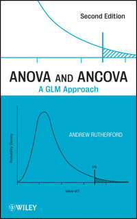
The purpose of calculating an F-value is to determine whether the differences between the experimental condition means are significant. This is accomplished by comparing the calculated F-value with the sampling distribution of the F-statistic. The F-statistic sampling distribution reflects the probability of different F-values occurring when the null hypothesis is true. The null hypothesis states that no differences exist between the means of the experimental condition populations. If the null hypothesis is true and the sample of subjects and their scores accurately reflect the population under the null hypothesis, then between group and within group variation estimates will be equal and the calculated F-value will equal 1. However, due to chance sampling variation (sometimes called sampling error), it is possible to observe differences between the experimental condition means of the data samples.

Figure 2.1 A typical distribution of F under the null hypothesis.

BOX 2.1

The F