111,99 €
Mehr erfahren.
- Herausgeber: John Wiley & Sons
- Kategorie: Wissenschaft und neue Technologien
- Sprache: Englisch
An Innovative Approach to Multidimensional Signals and Systems Theory for Image and Video Processing
In this volume, Eric Dubois further develops the theory of multi-D signal processing wherein input and output are vector-value signals. With this framework, he introduces the reader to crucial concepts in signal processing such as continuous- and discrete-domain signals and systems, discrete-domain periodic signals, sampling and reconstruction, light and color, random field models, image representation and more.
While most treatments use normalized representations for non-rectangular sampling, this approach obscures much of the geometrical and scale information of the signal. In contrast, Dr. Dubois uses actual units of space-time and frequency. Basis-independent representations appear as much as possible, and the basis is introduced where needed to perform calculations or implementations. Thus, lattice theory is developed from the beginning and rectangular sampling is treated as a special case. This is especially significant in the treatment of color and color image processing and for discrete transform representations based on symmetry groups, including fast computational algorithms. Other features include:
- An entire chapter on lattices, giving the reader a thorough grounding in the use of lattices in signal processing
- Extensive treatment of lattices as used to describe discrete-domain signals and signal periodicities
- Chapters on sampling and reconstruction, random field models, symmetry invariant signals and systems and multidimensional Fourier transformation properties
- Supplemented throughout with MATLAB examples and accompanying downloadable source code
Graduate and doctoral students as well as senior undergraduates and professionals working in signal processing or video/image processing and imaging will appreciate this fresh approach to multidimensional signals and systems theory, both as a thorough introduction to the subject and as inspiration for future research.
Sie lesen das E-Book in den Legimi-Apps auf:
Seitenzahl: 443
Veröffentlichungsjahr: 2019
Ähnliche


Multidimensional Signal and Color Image Processing Using Lattices
Eric Dubois
University of Ottawa
Copyright
This edition first published 2019
© 2019 John Wiley & Sons, Ltd
All rights reserved. No part of this publication may be reproduced, stored in a retrieval system, or transmitted, in any form or by any means, electronic, mechanical, photocopying, recording or otherwise, except as permitted by law. Advice on how to obtain permission to reuse material from this title is available at http://www.wiley.com/go/permissions.
The right of Eric Dubois to be identified as the author of this work has been asserted in accordance with law.
Registered Office(s)
John Wiley & Sons, Inc., 111 River Street, Hoboken, NJ 07030, USA
John Wiley & Sons Ltd, The Atrium, Southern Gate, Chichester, West Sussex, PO19 8SQ, UK
Editorial Office
The Atrium, Southern Gate, Chichester, West Sussex, PO19 8SQ, UK
For details of our global editorial offices, customer services, and more information about Wiley products visit us at www.wiley.com.
Wiley also publishes its books in a variety of electronic formats and by print‐on‐demand. Some content that appears in standard print versions of this book may not be available in other formats.
Limit of Liability/Disclaimer of Warranty
While the publisher and authors have used their best efforts in preparing this work, they make no representations or warranties with respect to the accuracy or completeness of the contents of this work and specifically disclaim all warranties, including without limitation any implied warranties of merchantability or fitness for a particular purpose. No warranty may be created or extended by sales representatives, written sales materials or promotional statements for this work. The fact that an organization, website, or product is referred to in this work as a citation and/or potential source of further information does not mean that the publisher and authors endorse the information or services the organization, website, or product may provide or recommendations it may make. This work is sold with the understanding that the publisher is not engaged in rendering professional services. The advice and strategies contained herein may not be suitable for your situation. You should consult with a specialist where appropriate. Further, readers should be aware that websites listed in this work may have changed or disappeared between when this work was written and when it is read. Neither the publisher nor authors shall be liable for any loss of profit or any other commercial damages, including but not limited to special, incidental, consequential, or other damages.
Library of Congress Cataloging‐in‐Publication Data
Names: Dubois, E. (Eric), author.
Title: Multidimensional signal and color image processing using lattices / Eric Dubois.
Description: Hoboken, NJ : John Wiley & Sons, 2019. | Includes bibliographical references and index. |
Identifiers: LCCN 2018048220 (print) | LCCN 2019002308 (ebook) | ISBN 9781119111757 (Adobe PDF) | ISBN 9781119111764 (ePub) | ISBN 9781119111740 (hardcover)
Subjects: LCSH: Signal processing. | Lattice theory. | Image processing–Mathematics.
Classification: LCC TK5102.9 (ebook) | LCC TK5102.9 .D83 2019 (print) | DDC 621.382/201511332–dc23
LC record available at https://lccn.loc.gov/2018048220
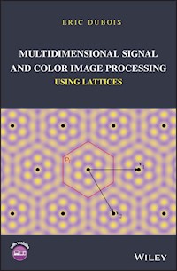
Cover image: Courtesy of Eric Dubois
To Sheila
About the Companion Website
The supplementary material is available on an accompanying website
www.wiley.com/go/Dubois/multiSP.
1Introduction
This book presents the theory of multidimensional (multiD) signals and systems, primarily in the context of image and video processing. MultiD signals are considered to be functions defined on some domain of dimension two or higher with values belonging to a set , the range. These values may represent the brightness or color of an image or some other type of measurement at each point in the domain. With this interpretation, a multiD signal is represented as
i.e. each element of the domain is mapped to the value belonging to the range . In conventional continuous‐time one‐dimensional (1D) signals and systems theory [Oppenheim and Willsky (1997)], and are both the set of real numbers , and so a real 1D signal would be written , . MultiD signals arise when the domain is a space with two or more dimensions. The domain can be continuous, as in the case of real‐world still and time‐varying images, or discrete, as in the case of sampled images. In addition, the range can also be a higher‐dimensional space, for example the three‐dimensional color space of human vision.
In this book, we are mainly concerned with examples from conventional still and time‐varying images, although the theory has broader applicability. A conventional planar image is written , where lies in a planar region associated with the Euclidean space . Here, denotes the horizontal spatial position and is the vertical spatial position while denotes image brightness or color. The domain can be itself, or a discrete subset in the case of sampled images. Similarly, a conventional time‐varying image is written , where lies in a subset (possibly discrete) of , which may also be written . Here, and are as above, and represents time. Higher‐dimensional cases also exist, for example time‐varying volumetric images with and where denotes some measurement taken at location at time . The domain can also be a more complicated manifold such as a cylinder or a sphere, as in panoramic imaging.
MultiD signal processing has been an active area of study for over fifty years. Early work was in optics and the continuous domain. Papoulis's classic text on Systems and Transforms with Applications in Optics appeared in 1968 [Papoulis (1968)]. Soon after, work on two‐dimensional digital filtering started to appear, for example [Hu and Rabiner (1972)]. Over the years, there have been several books devoted to multiD digital signal processing and numerous books on image and video processing. The present book is distinguished from these works in a number of aspects. The book is mainly concerned with the theory of discrete‐domain processing of real‐ or vector‐valued multiD signals. The application examples are drawn from grayscale and color image processing and video processing. In particular, the book is not intended to present the state‐of‐the‐art algorithms for particular image processing tasks.
Most previous books on multiD signals considered rectangularly sampled signals for the main development and presented non‐rectangular sampling on a lattice as a subsidiary extension. A lattice, as in crystal lattice, is a mathematical structure from which we can construct more general sampling structures. In this book, the theory is developed on lattices from the beginning, and rectangular sampling is considered a special case. Another difference is that most books use normalized representations for non‐rectangular sampling that are dependent on the lattice basis. Although this may be convenient for certain manipulations, this approach obscures much of the geometrical and scale information of the signal. We prefer to use basis‐independent representations as much as possible, and introduce the basis where needed to perform calculations or implementations. Thus, we do not use such normalized representations but rather use the actual units of space‐time and frequency.
Another distinguishing feature of this book is the treatment of color. Color signals are viewed as multiD signals with values in a vector space, in this case the vector space of human color vision, and color signal processing is viewed as vector‐valued signal processing. Most multiD signal processing books deal mainly with scalar signals, representing a grayscale or brightness value. If color models are introduced, color signal processing generally involves separate processing of three color channels. Here we present the theory of multiD signal processing where the input and output are vector‐valued signals, further developing the theory introduced in Dubois (2010).
In general, multiD signals in the real world, such as still and time‐varying images, are functions of the continuous space and time variables. Consider for example a light signal falling on a camera sensor or emanating from a motion‐picture screen. These multiD signals are converted to discrete‐domain signals for digital processing, storage, and transmission. They may eventually be converted back to continuous‐domain signals, for example for viewing on a display device. Thus, we begin with an overview of scalar‐valued continuous‐domain multiD signals and systems, i.e. the domain is for some integer . In particular we introduce the concepts of signal space, linear shift‐invariant systems and the continuous‐domain multiD Fourier transform, develop properties of the Fourier transform and present some examples. Continuous‐domain signal spaces and transforms involve advanced mathematical analysis to provide a general theory for arbitrary signal spaces. We do not attempt to provide a rigorous analysis. We assume that signals belong to a suitable signal space for which transforms are well defined and the properties hold. For example, a space of tempered distributions would be satisfactory. However, we do not develop the theory of distributions and take an informal approach to the Dirac delta and related singularities. We refer the reader to references for a rigorous analysis, e.g., [Stein and Weiss (1971), Richards and Youn (1990)].
There are many possible domains for multiD signals, generally subsets of for some . These domains can be continuous or discrete, or a hybrid that is continuous in some dimensions and discrete in others, like in analog TV scanning. The domain can also correspond to one period of a periodic signal, whether continuous or discrete. Among the possible domains, certain of them allow for the possibility of linear shift‐invariant filtering. These domains have the algebraic structure of a locally‐compact Abelian (LCA) group. While we cannot go into the detail of such structures, their main feature is that the concept of shift is well defined and commutative. is an example, as is any lattice in . The LCA group is the classical setting for abstract harmonic analysis, e.g., as presented in Rudin (1962). An early work on signal processing in this setting is the Ph.D. thesis of Rudolph Seviora [Seviora (1971)]), which considered generalized digital filtering on LCA groups. More recently Cariolaro has developed signal processing on LCA groups in a comprehensive book [Cariolaro (2011)].
In this book, we have elected to provide a separate development for the cases of continuous‐domain aperiodic signals, discrete‐domain aperiodic signals, discrete‐domain periodic signals, and continuous‐domain periodic signals (Chapters 02–05). Each case has its own sphere of application, and while the development may be redundant from an abstract mathematical perspective, the concrete details are sufficiently different to warrant their own presentation. Each of these chapters follows a similar roadmap, presenting concepts of signal space, linear shift‐invariant (LSI) systems, Fourier transforms and their properties. For discrete‐domain signals, we use lattices to describe the sampling structure. For periodic signals, we use lattices to describe the periodicity. Since lattices form an underlying tool used throughout the book, we have chosen to gather all definitions and results about lattices that we need for this work in Chapter 13, which may be consulted any time as needed. We prefer not to interrupt the flow of the book at the beginning with this material, and we wish to give it a higher status than an appendix. This is why we have chosen to include it as the last chapter in the book.
In Chapter 6 we see the relationship between the four representations. Discrete‐domain aperiodic and periodic signals can be obtained for the corresponding continuous‐domain signals by a sampling operation. This is shown to induce a periodization in the frequency domain. In another view, discrete and continuous‐domain periodic signals can be obtained by periodization of corresponding aperiodic signals, resulting in sampling in the frequency domain. These results are all explored in Chapter 06and various sampling theorems are presented. We do not explicitly explore hybrid signals, which may correspond to a different one of the above types in different dimensions. This extension is usually straightforward; many examples are given in Cariolaro ( 2011).
Having developed the theory of processing of multiD scalar signals, we address the nature of the signal range in Chapter 7 , specifically for color image signals. Here we take up the vector‐space view of color spaces as presented in Dubois (2010), where colors are viewed as equivalence classes of light spectral densities that give the same response to a viewer. This viewer can be a typical human with a three‐dimensional color space or maybe a camera, which could have a higher‐dimensional color space. With this representation, we develop signal processing theory for color signals in Chapter 8 , again taking up and extending the presentation of Dubois (2010). Such a unified theory of color signal processing has not yet been widely adopted in the literature. One unique aspect is that color signals can have different sampling structures for different subspaces of the color space, as in the Bayer color filter array (CFA) of digital cameras, for example. This aspect is developed in Chapter 08.
MultiD signals can often be usefully considered to be realizations of a random process. This concept has been used extensively in multiD signal processing applications using many types of random field models. In Chapter 9 , we present some basic concepts on multiD random fields, limiting the presentation to wide‐sense stationary random fields characterized by correlation functions and spectral densities. One novel aspect is the development of vector‐valued random field models for color signals. Most books on random processes deal mainly with scalar signals, and may just mention the case of vector signals (e.g., Leon‐Garcia (2008), Stark and Woods (2002)). However, some classic texts (e.g., Brillinger (2001), Priestley (1981)) consider vector‐valued random processes in detail and we follow this approach for correlation functions and spectral densities of color or other vector‐valued signals. However, we do not go into more elaborate random field models such as Gibbs–Markov random fields, which have been very successful. These are covered in several books, including for example Fieguth (2011).
In Chapter 10 , we present some multiD filter design methods and examples, and then consider the specific example of change of sampling structure of an image in Chapter 11. These developments are all carried out in the general context of lattices. We do not delve into general multiD multiresolution signal processing such as filter banks in this book. This topic can also be developed using a general lattice formulation, such as in our previous work [Coulombe and Dubois (1999)], or in the works by Suter (1998) and Do and Lu (2011).
We then present a novel development of symmetry‐invariant signals and systems in Chapter 12. This extends the concept of linear shift‐invariant systems to systems invariant to other transformations of Euclidean space, such as rotations and reflections. This uses the theory of symmetry groups, widely used in fields such as crystallography. One outcome of this development is the generalization of the widely used separable discrete cosine transform (DCT) to arbitrary lattices.
As mentioned above, Chapter 13 gathers all the material and results on lattices used throughout the book into a single chapter, which can stand alone. This is followed by some brief appendices describing a few aspects of equivalence relations, groups and vector spaces. One should consult suitable textbooks on algebra, such as the ones cited, for a complete presentation of these topics. Throughout the book, all results requiring a proof have been called theorems regardless of their importance, rather than trying to categorize them as theorem, proposition, lemma, etc.
Most of the material in this book (other than Chapter 12
2Continuous‐Domain Signals and Systems
2.1 Introduction
This chapter presents the relevant theory of continuous‐domain signals and systems, mainly as it applies to still and time‐varying images. This is a classical topic, well covered in many texts such as Papoulis's treatise on Systems and Transforms with Applications in Optics [Papoulis (1968)] and the encyclopedic Foundations of Image Science [Barrett and Myers (2004)]. The goal of this chapter is to present the necessary material to understand image acquisition and reconstruction systems, and the relation to discrete‐domain signals and systems. Fine points of the theory and vastly more material can be found in the cited references.
A continuous‐domain planar time‐varying image is a function of two spatial dimensions and , and time , usually observed in a rectangular spatial window over some time interval . In the case of a still image, has a constant value for each , independently of . In this case, we usually suppress the time variable, and write . We use a vector notation to simplify the notation and handle two and three‐dimensional (and higher‐dimensional) cases simultaneously. Thus is understood to mean in the two‐dimensional case and in the three‐dimensional case. We will denote and , where is the set of real numbers. To cover both cases, we write , where normally or ; also the one‐dimensional case is covered with and most results apply for dimensions higher than 3. For example, the domain for time‐varying volumetric images is . It is often convenient to express the independent variables as a column matrix, i.e.
Since there is no essential difference between and the space of column matrices, we do not distinguish between these different representations. We will often abbreviate two‐dimensional as 2D and three‐dimensional as 3D.
The spatial window is of dimensions where pw is the picture width and ph is the picture height. Since the absolute physical size of an image depends on the sensor or display device used, we often choose to adopt the ph as the basic unit of spatial distance, as has long been common in the broadcast video industry. However, we are free to choose any convenient unit of length in a given application, for example, the size of a sensor or display element, or an absolute measure of distance such as the meter or micron. The ratio is called the aspect ratio, the most common values being 4/3 for standard TV and 16/9 for HDTV. With this notation, ph (see Figure 2.1). Time is measured in seconds, denoted s. Examples of continuous‐domain space‐time images include the illumination on the sensor of a video camera, or the luminance of the light reflected by a cinema screen or emitted by a television display.
Since the image is undefined outside the spatial window , we are free to extend it outside the window as we see fit to include all of as the domain. Some possibilities are to set the image to zero outside , to periodically repeat the image, or to extrapolate it in some way. Which of these is chosen depends on the application.
Figure 2.1 Illustration of image window with aspect ratio ph.
There are two common ways to attach an coordinate system to the image window, involving the location of the origin and the orientation of the and axes, as shown in Figure 2.2. The standard orientation used in mathematics to graph functions would place the origin at the lower left corner of the image with the ‐axis pointing upward. However, because traditionally images have been scanned from top to bottom, most image file formats store the image line‐by‐line, with the top line first, and line numbers increasing from top to bottom of the image. This makes the orientation shown in Figure 2.2(b) more convenient, with the origin in the upper left corner of the image and the ‐axis pointing downward. For this reason, we will generally use the orientation of Figure 2.2(b).
Figure 2.2 Orientation of ‐axes. (a) Common bottom‐to‐top orientation in mathematics. (b) Scanning‐based top‐to‐bottom orientation.
2.2 Multidimensional Signals
A multiD signal can be considered to be a function from the domain, here , to the range. In this and the next few chapters, we consider only real and complex valued signals, which we call scalar signals. In later chapters, where we consider color signals, we will take the range to be a suitable vector space. In addition to naturally occurring continuous space‐time images, many analytically defined ‐dimensional functions are useful in image processing theory. A few of these are introduced here.
2.2.1 Zero–One Functions
Let be a region in the ‐dimensional space, . We define the zero–one function as illustrated in Figure 2.3(a) by
Sometimes, is called the indicator function of the region . Different functions are obtained with different choices of the region . Such functions arise frequently in modeling sensor elements or display elements (sub‐pixels). The most commonly used ones in image processing are the rect and the circ functions in two dimensions. Specifically, for a unit‐square region we obtain (Figure 2.3(b))
For a circular region of unit radius we have (Figure 2.3(c))
These definitions can be extended to the three‐dimensional case (where the region is a cube or a sphere) or to higher dimensions in a straightforward fashion, and the single notation or can be used to cover all cases. We will see later how these basic signals can be shifted, scaled, rotated or otherwise transformed to generate a much richer set of zero–one functions. Other zero–one functions that we will encounter correspond to various polygonal regions such as triangles, hexagons, octagons, etc.
Figure 2.3 Zero–one functions. (a) General zero–one function. (b) Rect function. (c) Circ function.
2.2.2 Sinusoidal Signals
As in one‐dimensional signals and systems, real and complex‐exponential sinusoidal signals play an important role in the analysis of image processing systems. There are several reasons for this but a principal one is that if a complex‐exponential sinusoidal signal is applied as input to a linear shift‐invariant system (to be introduced shortly), the output is equal to the input multiplied by a complex scalar. A general, real two‐dimensional sinusoid with spatial frequency is given by
where and are spatial coordinates in ph (say), and are fixed spatial frequencies in units of c/ph (cycles per picture height) and is the phase. In general, for a given unit of spatial distance (e.g., m), spatial frequencies are measured in units of cycles per said unit (e.g., c/m).
Figure 2.4 illustrates a sinusoidal signal with horizontal frequency 1.5 c/ph and vertical frequency 2.5 c/ph in a square image window of size 1 ph by 1 ph. The actual signal displayed is , which has a range from 0 (black) to 1 (white). From this figure, we can identify a number of features of the spatial sinusoidal signal. The sinusoidal signal is periodic in both the horizontal and vertical directions, with horizontal period and vertical period . The signal is constant if is constant, i.e. along lines parallel to the line .
The one‐dimensional signal along any line through the origin is a sinusoidal function of distance along the line. The maximum frequency along any such line is , along the line , as illustrated in Figure 2.4. The proof is left as an exercise.
Figure 2.4 Sinusoidal signal with = 1.5 c/ph and = 2.5 c/ph. The horizontal period is (2/3) ph and the vertical period is 0.4 ph. The frequency along the line is 2.9 c/ph, corresponding to a period of 0.34 ph.
As in one dimension, the complex exponential sinusoidal signals play an important role, e.g., in Fourier analysis. The complex exponential corresponding to the real sinusoid of Equation (2.4) is
where can be complex. In this book, we use j to denote . We often will adopt the vector notation
where in the two‐dimensional case denotes as before, denotes and denotes . When using the column matrix notation, then and we can write . This is extended to any number of dimensions in a straightforward manner. Using Euler's formula, the complex exponential can be written in terms of real sinusoidal signals
If is given as in Equation (2.6), then for any fixed , we have
In other words, the shifted complex exponential is equal to the original complex exponential multiplied by the complex constant . This in turn leads to the key property of linear shift‐invariant systems mentioned earlier in this section. This will be analyzed in Section 2.5.5 but is mentioned here to motivate the importance of sinusoidal signals in multidimensional signal processing.
2.2.3 Real Exponential Functions
Real exponential signals also have wide applicability in multidimensional signal processing. First‐order exponential signals are given by
and second‐order, or Gaussian, signals by
Gaussian signals, similar in form to the Gaussian probability density, are widely used in image processing. Some illustrations can be seen later, in Figure 2.6. We define the standard versions of these signals as follows:
2.2.4 Zone Plate
A very useful two‐dimensional function that is often used as a test pattern in imaging systems is the zone plate, or Fresnel zone plate. The sinusoidal zone plate is based on the function
where is a parameter that sets the scale. Figure 2.5 illustrates the zone plate with ph. It is often convenient to consider the zone plate as the real part of the complex exponential function .
Figure 2.5 Illustration of a zone plate with parameter ph. Local horizontal and vertical frequencies range from 0 to 125 c/ph.
Examining Figure 2.5, it can be seen that locally (say, within a small square window) the function is a sinusoidal signal with a horizontal frequency that increases with horizontal distance from the origin, and similarly a vertical frequency that increases with vertical distance from the origin. To make this concept of local frequency more precise, consider a conventional two‐dimensional sinusoidal signal
where . In this case we see that the horizontal and vertical frequencies are given by
We use these definitions to define the local frequency of a generalized sinusoidal signal . For the zone plate, we have and so obtain
which confirms that local horizontal and vertical frequencies vary linearly with horizontal and vertical position respectively.
We define standard versions of the real and complex zone plates by


