66,99 €
Mehr erfahren.
- Herausgeber: John Wiley & Sons
- Kategorie: Wissenschaft und neue Technologien
- Sprache: Englisch
Professionals in all areas – business; government; the physical, life, and social sciences; engineering; medicine, etc. – benefit from using statistical experimental design to better understand their worlds and then use that understanding to improve the products, processes, and programs they are responsible for. This book aims to provide the practitioners of tomorrow with a memorable, easy to read, engaging guide to statistics and experimental design.
This book uses examples, drawn from a variety of established texts, and embeds them in a business or scientific context, seasoned with a dash of humor, to emphasize the issues and ideas that led to the experiment and the what-do-we-do-next? steps after the experiment. Graphical data displays are emphasized as means of discovery and communication and formulas are minimized, with a focus on interpreting the results that software produce. The role of subject-matter knowledge, and passion, is also illustrated. The examples do not require specialized knowledge, and the lessons they contain are transferrable to other contexts.
Fundamentals of Statistical Experimental Design and Analysis introduces the basic elements of an experimental design, and the basic concepts underlying statistical analyses. Subsequent chapters address the following families of experimental designs:
- Completely Randomized designs, with single or multiple treatment factors, quantitative or qualitative
- Randomized Block designs
- Latin Square designs
- Split-Unit designs
- Repeated Measures designs
- Robust designs
- Optimal designs
Written in an accessible, student-friendly style, this book is suitable for a general audience and particularly for those professionals seeking to improve and apply their understanding of experimental design.
Sie lesen das E-Book in den Legimi-Apps auf:
Seitenzahl: 474
Veröffentlichungsjahr: 2015
Ähnliche


Table of Contents
Cover
Title Page
Preface
References
Statistical Software
Sources for Student Exercises (in addition to the above references)
Acknowledgments
Credits
1 Introduction
Motivation: Why Experiment?
Steps in an Experimental Program
Subject-Matter Passion
Case Study
Overview of Text
Assignment
References
2 Fundamentals of Experimental Design
Introduction
Experimental Structure
Principles of Experimental Design
Assignment
References
3 Fundamentals of Statistical Data Analysis
Introduction
Boys’ Shoes Experiment
Tomato Fertilizer Experiment
A New Tomato Experiment
Comparing Standard Deviations
Discussion
Appendix 3.A The Binomial Distribution
Appendix 3.B Sampling from a Normal Distribution
Appendix 3.C Statistical Underpinnings
Assignment
References
4 Completely Randomized Design
Introduction
Design Issues
CRD: Single
Qualitative
Factor
Analysis of Variance
Testing the Assumptions of Equal Variances and Normality
Confidence Intervals
Inference
Statistical Prediction Interval
Example: Tomato Fertilizer Experiment Revisited
Sizing a Completely Randomized Experiment
CRD: Single Quantitative Factor
Design Issues
Enhanced Case Study: Power Window Gear Teeth
Assignment
References
5 Completely Randomized Design with Multiple Treatment Factors
Introduction
Design Issues
Response Surface Designs
Special Case: Two-Level Factorial Experiments
Fractional
Two-Level Factorials
Extensions
Assignment
References
6 Randomized Complete Block Design
Introduction
Design Issues
RBD with Single Replication
Sizing a Randomized Block Experiment
True Replication
Extensions of the RBD
Discussion
Balanced Incomplete Block Designs
Summary
Assignment
References
7 Other Experimental Designs
Introduction
Latin Square Design
Split-Unit Designs
Repeated Measures Designs
Robust Designs
Optimal Designs
Assignment
References
Index
End User License Agreement
List of Tables
Chapter 03
Table 3.1 Boys’ Shoes Example: Percent Wear for Soles of Materials A and B; Material A on the Indicated Foot.
Table 3.2 Minitab Output for Paired
t
-Test: Boys’ Shoes.
Table 3.3 Excel Paired
t
-Test Analysis of the Boys’ Shoe Data.
Table 3.4 Results of Tomato Fertilizer Experiment.
Table 3.5 Results of Year 2 Tomato Experiment.
Table 3.6 Minitab Output: Tomato Fertilizer Experiment 2: Two-Sample
t
-Test Assuming Equal Variances.
Table 3.7 Minitab Analysis of Tomato Experiment 2: Two-Sample
t
-Test Assuming Unequal Variances.
Table 3.8 Minitab Output: Power and Sample Size.
Chapter 04
Table 4.1 Sales Data: %Increase in Sales for Four Displays. Each display was installed in five different stores for 1 week.
Table 4.2 Analysis of Variance (ANOVA) Table for the Completely Randomized Design: One Treatment Factor with
k
Levels and
n
Observations per Treatment.
Table 4.3 ANOVA of SalesIncr% Data.
Table 4.4 ANOVA for Tomato Fertilizer Experiment 2.
Table 4.5 Regression Analysis Results.
Table 4.6 ANOVA for Quadratic Model.
Table 4.7 Gear Teeth Data and Schematic.
Table 4.8 ANOVA of Gear Teeth Impact Strength Data.
Chapter 05
Table 5.1 Animal Survival Times (in tenths of hour).
Table 5.2 Average Death Rates (units of hour
−1
) by Poisons and Antidotes.
Table 5.3 ANOVA for Death Rate.
Table 5.4 Weights in Estimated Mean Death Rate: Poison III, Antidote B.
Table 5.5 Regression Analysis of CO Emissions Data.
Table 5.6 ANOVA for CO Quadratic Model.
Table 5.7 Response Surface Design for Two
x
-Variables.
Table 5.8 ANOVA for Poison/Antidote/Delay/Dosage Experiment.
Table 5.9 Pot Production Experimental Results.
Table 5.10 Main Effect and Two-Factor Interaction Variables in Regression Analysis.
Table 5.11 Fitted Coefficients for a Full Four-Factor Model.
Table 5.12 Effects and Regression Coefficients for Flower Pot Experiment.
Table 5.13 Regression Variables in 2
4
Factorial Treatment Design.
Table 5.14 Regression Variables in 1/2 of a 2
4
Factorial Treatment Design.
Chapter 06
Table 6.1 Battery Lifetimes by Material and Temperature.
Table 6.2 ANOVA Structure for Randomized Complete Block Design with Replication.
Table 6.3 ANOVA for Battery Experiment.
Table 6.4 ANOVA for Battery Experiment: Materials 2 and 3.
Table 6.5 Fahrenheit Temperatures Converted to Centigrade, Kelvin, and the Reciprocal of Kelvin Temperature.
Table 6.6 Two-Way ANOVA: Yield versus Batch, Process.
Table 6.7 One-Way ANOVA: Penicillin Yield versus Batch.
Table 6.8 ANOVA for Modified Battery Experiment.
Table 6.9 Two-Way ANOVA: Wear % versus Boy No., Material.
Table 6.10 ANOVA for Penicillin Experiment, Extended.
Chapter 07
Table 7.1 4 × 4 Latin Square Design for Additive Experiment.
Table 7.2 Results of Car Emission Latin Square Experiment.
Table 7.3 ANOVA for Emissions Experiment.
Table 7.4 Reduced ANOVA of Emissions Data.
Table 7.5 4 × 4 Graeco-Latin Design.
Table 7.6 Corrosion-Resistance Experiment Data.
Table 7.7 ANOVA Structure for Corrosion-Resistance Experiment.
Table 7.8 ANOVA for Corrosion-Resistance Split-Unit Experiment.
Table 7.9
Incorrect ANOVA
of Corrosion-Resistance Experiment: Split-Unit Design Structure
Not
Recognized.
Table 7.10 Heart Rate Data.
Table 7.11 ANOVA for Drug/Pulse Rate Experiment.
List of Illustrations
Chapter 01
Figure 1.1 Statistics Schematic.
Figure 1.2 Car Data: Engine Size versus Body Weight.
Figure 1.3 Bond-Strength Distribution.
Figure 1.4 Average Bond Strengths by Bonding and Pull-Test Operators.
Chapter 02
Figure 2.1 Nested Experimental Unit Structure.
Figure 2.2 Crossed and Nested Combinations of Treatment Factors. The three levels of B are different at the three levels of A; B is nested in A.
Figure 2.3 (a) Completely Randomized Assignment of Treatments. (b) Random Assignment of Treatments within Each Block (Day).
Chapter 03
Figure 3.1 Scatter Plot of B-Material Wear versus A-Material Wear; separate plotting symbols for the left and right foot assignments of material A.
Figure 3.2 Wear % by Material and Boy.
Figure 3.3 Line Plot of Wear Data for Materials A and B.
Figure 3.4 Binomial Distribution.
B
(
x
:10, .5) denotes the probability of
x
heads in 10 fair tosses of a fair coin.
Figure 3.5 Comparison of Shoe Experiment Results to the Binomial Distribution for
n
= 10,
p
= .5.
Figure 3.6 The Standard Normal Distribution. Statistical convention is to denote a variable that has the standard normal distribution by
z
.
Figure 3.7 Individual Value Plot of Shoe-Wear Differences (%). The average difference is indicated by the blue symbol.
Figure 3.8 Comparison of the Observed
t
-Value (3.4) to the
t
-Distribution with 9
df.
Figure 3.9 Illustration of Confidence Interval: Boys’ Shoes Experiment.
Figure 3.10 Data from Tomato Fertilizer Experiment. Yield, in pounds, is plotted versus row position, by fertilizer.
Figure 3.11 Tomato Yield by Position and Fertilizer: Experiment 2.
Figure 3.12 Dot Plot of Yields by Fertilizer: Experiment 2.
Figure 3.13 Reference Distribution for the Rank Sum Statistic: Tomato Experiment 2.
Figure 3.14 Randomization Distribution of Average Difference Between Fertilizers in Tomato Experiment 2: C–A. Plot produced by Stat101 software (Simon 1997).
Figure 3.15 Tomato Experiment 2. Comparison of the observed
t
-statistic to the
t
(14)-distribution.
Figure 3.16 Power Curve for the Plan Determined in Table 3.8.
Figure 3.17 Power Curves for Different Sample Sizes.
Figure 3.18 Comparison of
F
-Statistic for Experiment 2 to the
F
(7, 7) Distribution.
Figure 3.19 Two-Tail
F
-Test for Comparing Variances for Fertilizers A and C.
Figure 3.A.1 Binomial Distribution for
n
= 10,
p
= .2. The observed outcome,
x
= 2, is the most likely value in this distribution.
Figure 3.A.2 (a) Binomial Distribution for
n
= 10,
p
= .037. (b) Binomial Distribution for
n
= 10,
p
= .051.
Figure 3.B.1 Ten Random Samples of 10 Observations from a Normal Distribution.
Figure 3.B.2 Dot Plot of Boys’ Shoe Data.
Figure 3.B.3 Probability Plot of Boys’ Shoes Data.
Chapter 04
Figure 4.1 Pct. Increase of Shampoo Sales by Display.
Figure 4.2 Graphical
F
-Test for Testing the Hypothesis of No Difference Among the Underlying Means for
k
Treatment Groups.
Figure 4.3 Graphical Depiction of
F
-Test for Shampoo Sales Experiment.
Figure 4.4 Data from Growth Rate Experiment. Source: Box, Hunter, and Hunter (2005, p. 381), used here by permission of John Wiley & Sons.
Figure 4.5 Data Plot and Fitted Model.
Figure 4.6 Fitted Model with 95% Confidence Intervals on the Underlying Expected Growth Rate as a Function of Amount of Supplement.
Figure 4.7 Box and Whisker Plot of Impact Strength Data.
Figure 4.8 Average Impact Strengths by Position.
Chapter 05
Figure 5.1 Data Plot: Poison—Antidote Experiment.
Figure 5.2 Plot of Death Rates versus Antidotes, by Poisons.
Figure 5.3 Interaction Plot. Average death rate versus poison, by antidote.
Figure 5.4 Interaction Plot. Average death rate versus antidote, by poison.
Figure 5.5 Antidote Average Death Rates.
Figure 5.6 Estimated Survival Curve and 95% Statistical Confidence Intervals.
Figure 5.7 Plots of CO versus
x
1, by Values of
x
2.
Figure 5.8 Plots of CO versus
x
2, by Values of
x
1.
Figure 5.9 Interaction Plots for Ethanol Experiment.
Figure 5.10 Average CO Emissions by
x
1,
x
2 Combinations.
Figure 5.11 Contour Plot of CO versus
x
1 and
x
2.
Figure 5.12 Scatter Plot of Observed CO Values versus Fitted Values.
Figure 5.13 Response Surface Design for Two
x
-Variables in Coded Units. 2 × 2 factorial points connected by black lines; “star” points connected by blue lines; axial points at ±1.4.
Figure 5.14 Interaction Plot for Factors
R
and
C
.
Figure 5.15 Dot Plot of Coefficients.
Figure 5.16 Normal Probability Plot of Estimated Coefficients.
Figure 5.17 Normal Probability Plot of Effects and Interactions.
Figure 5.18 Schematic of One-Factor-at-a-Time Experiment: Three Two-Level Factors.
Figure 5.19 Schematic of Fractional Factorial Experiment: Three Two-Level Factors.
Figure 5.20 Graphical Analysis of 1/2 Fraction:
RTCD
= 1.
Figure 5.21 Graphical Analysis of 1/2 Fraction:
RTCD
= −1.
Chapter 06
Figure 6.1 Scatter Plot of Battery Lifetimes versus Temperature, by Material.
Figure 6.2 Interaction Plot of Material/Temperature Means.
Figure 6.3 Plot of Average Log-Lifetimes versus Inverse Absolute Temperature.
Figure 6.4 Data Plot for Penicillin Yield Experiment. .
Figure 6.5 Penicillin Yields by Batch.
Figure 6.6 Cloth Strength by Technicians and Looms. Source: Scott and Triggs (2003, p. 91), used here by permission of Department of Statistics, University of Auckland.
Chapter 07
Figure 7.1 Average Emissions by Car, Driver, and Additive.
Figure 7.2 Interaction Plot of Emissions Data by Additive and Driver.
Figure 7.3 Schematic Illustrating Split-Unit Design for Tomato Fertilizer Experiment. The design has 20 main-plot units, with each fertilizer randomly assigned to 10 units. Each main-plot unit is divided into three subplots, and the three fertilizer levels are randomly assigned to one subplot unit each.
Figure 7.4 Corrosion Resistance Plotted as a Function of Heat, Curing Temperature, and Coating.
Figure 7.5 Plot of Corrosion Resistance versus Curing Temperature by Coating.
Figure 7.6 Interaction Plot of Corrosion Resistance Averages versus Temperature by Coating.
Figure 7.7 Plot of Pulse Rate versus Time (min) by Subject and Drug.
Figure 7.8 Average Pulse Rate versus Time by Drug.
Figure 7.9 The Transmission of Variation in the Length of a Pendulum to Variability of the Pendulum’s Period. .
Figure 7.10 An Inner 3 × 3 Array of Two Design Factors and an Outer 2
3
Array of Three Noise Factors. .
Guide
Cover
Table of Contents
Begin Reading
Pages
ii
iii
iv
v
xiii
xiv
xv
xvi
xvii
xix
xxi
1
2
3
4
5
6
7
8
9
10
11
12
13
14
15
16
17
18
19
20
21
22
23
24
25
26
27
29
30
31
32
33
34
35
36
37
38
39
40
41
42
43
44
45
46
47
48
49
50
51
52
53
54
55
56
57
58
59
61
62
63
64
65
66
67
68
69
70
71
72
73
74
75
76
77
78
79
80
81
82
83
84
85
86
87
88
60
89
91
92
93
94
95
96
97
98
99
100
101
102
103
104
105
106
107
108
109
110
111
112
113
114
115
116
117
118
119
120
121
123
124
125
126
127
128
129
130
131
132
133
134
135
136
137
138
139
140
141
142
143
144
145
146
147
148
149
150
151
152
153
154
155
156
157
158
159
160
161
162
163
164
165
166
167
168
169
170
171
172
173
174
175
177
178
179
180
181
182
183
184
185
186
187
188
189
190
191
192
194
195
196
197
198
199
200
201
202
203
204
205
207
208
209
210
211
212
213
214
215
216
217
218
219
220
221
222
223
224
225
226
227
228
229
230
231
232
233
234
235
236
237
238
239
240
241
242
243
245
246
Fundamentals of Statistical Experimental Design and Analysis
Robert G. Easterling
Cedar Crest, New Mexico, USA
This edition first published 2015© 2015 John Wiley & Sons, Ltd
Registered OfficeJohn Wiley & Sons, Ltd, The Atrium, Southern Gate, Chichester, West Sussex, PO19 8SQ,United Kingdom
For details of our global editorial offices, for customer services and for information about how to apply for permission to reuse the copyright material in this book please see our website at www.wiley.com.
The right of the author to be identified as the author of this work has been asserted in accordance with the Copyright, Designs and Patents Act 1988.
All rights reserved. No part of this publication may be reproduced, stored in a retrieval system, or transmitted, in any form or by any means, electronic, mechanical, photocopying, recording or otherwise, except as permitted by the UK Copyright, Designs and Patents Act 1988, without the prior permission of the publisher.
Wiley also publishes its books in a variety of electronic formats. Some content that appears in print may not be available in electronic books.
Designations used by companies to distinguish their products are often claimed as trademarks. All brand names and product names used in this book are trade names, service marks, trademarks or registered trademarks of their respective owners. The publisher is not associated with any product or vendor mentioned in this book.
Limit of Liability/Disclaimer of Warranty: While the publisher and author have used their best efforts in preparing this book, they make no representations or warranties with respect to the accuracy or completeness of the contents of this book and specifically disclaim any implied warranties of merchantability or fitness for a particular purpose. It is sold on the understanding that the publisher is not engaged in rendering professional services and neither the publisher nor the author shall be liable for damages arising herefrom. If professional advice or other expert assistance is required, the services of a competent professional should be sought
Library of Congress Cataloging-in-Publication Data
Easterling, Robert G. Fundamentals of statistical experimental design and analysis / Robert G. Easterling, Cedar Crest, New Mexico, USA. pages cm Includes bibliographical references and index.
ISBN 978-1-118-95463-8 (cloth)1. Mathematical statistics–Study and teaching. 2. Mathematical statistics–Anecdotes.3. Experimental design. I. Title.QA276.18.E27 2015519.5′7–dc23
2015015481
A catalogue record for this book is available from the British Library.
Dedications
Experimental Design Mentors, Oklahoma State UniversityDavid WeeksBob Morrison
Statistical Consulting Mentor, Sandia National LaboratoriesDick Prairie
Preface
I have a dream: that professionals in all areas—business; government; the physical, life, and social sciences; engineering; medicine; and others—will increasingly use statistical experimental design to better understand their worlds and to use that understanding to improve the products, processes, and programs they are responsible for. To this end, these professionals need to be inspired and taught, early, to conduct well-conceived and well-executed experiments and then properly extract, communicate, and act on information generated by the experiment. This learning can and should happen at the undergraduate level—in a way that carries over into a student’s eventual career. This text is aimed at fulfilling that goal.
Many excellent statistical texts on experimental design and analysis have been written by statisticians, primarily for students in statistics. These texts are generally more technical and more comprehensive than is appropriate for a mixed-discipline undergraduate audience and a one-semester course, the audience and scope this text addresses. Such texts tend to focus heavily on statistical analysis, for a catalog of designs. In practice, however, finding and implementing an experimental design capable of answering questions of importance are often where the battle is won. The data from a well-designed experiment may almost analyze themselves—often graphically. Rising generations of statisticians and the professionals with whom they will collaborate need more training on the design process than may be provided in graduate-level statistical texts.
Additionally, there are many experimental design texts, typically used in research methods courses in individual disciplines, that focus on one area of application. This book is aimed at a more heterogeneous collection of students who may not yet have chosen a particular career path. The examples have been chosen to be understandable without any specialized knowledge, while the basic ideas are transferable to particular situations and applications a student will subsequently encounter.
Successful experiments require subject-matter knowledge and passion and the statistical tools to translate that knowledge and passion into useful information. Archie Bunker, in the TV series, All in the Family, once told his son-in-law (approximately and with typical inadvertent profundity), “Don’t give me no stastistics (sic), Meathead. I want facts!” Statistical texts naturally focus on “stastistics”: here’s how to calculate a regression line, a confidence interval, an analysis of variance table, etc. For the professional in fields other than statistics, those methods are only a means to an end: revealing and understanding new facts pertinent to his or her area of interest. This text strives to make the connection between facts and statistics. Students should see from the beginning the connection between the statistics and the wider business or scientific context served by those statistics.
To achieve this goal, I tell stories about experiments, and bring in appropriate analyses, graphical and mathematical, as needed to move the stories along. I try to describe the situation that led to the experiment, what was learned, and what might happen after the experiment: “Fire the quality manager! Give the worthy statistician a bonus!” Experimental results need to be communicated in clear and convincing ways, so I emphasize graphical displays more than is often done in experimental design texts.
My stories are built around examples in statistical texts on experimental design, especially examples found in the classic text, Statistics for Experimenters, by Box, Hunter, and Hunter (1978, 2005). This “BHH” text has been on my desk since the first edition came out. I have taught several university classes based on it and have incorporated some of its material into my introductory statistics classes. Most of the examples are simple at first glance, but I have found it useful to (shamelessly) expand the stories in ways that address more of the design issues and more of the what-do-we-do-next issues. I try to make the stories provocative and entertaining because real-life experimentation is provocative and entertaining. I want the issues and concepts to be discussable by an interdisciplinary group of students and the lessons to be transferable to a student’s particular interests, with enough staying power to affect the student’s subsequent career. An underlying theme is that it is subject-matter enthusiasms that give rise to experiments, shape their design, and guide actions based on the findings. Statistical experimental design and data analysis methods facilitate and enhance the whole process. In short, statistics is a team sport. This text tries to demonstrate that.
In 1974, I taught at the University of Wisconsin and had the opportunity to attend the renowned Monday night “beer seminars” in the basement of the late Professor George Box’s home. He would invite researchers in to discuss their work, and the evening would turn into a grand consulting session among George, the researcher, and the students and faculty in attendance. The late Bill Hunter, also a professor in the Statistics Department and an innovative teacher of experimental design, was often a participant. I learned a lot in those sessions and hope that the atmosphere of those Monday night consulting sessions is reflected in the stories I have created here. The other H in BHH is J. Stuart Hunter, also an innovator in the teaching of experimental design; his presentations and articles have influenced me greatly, and his support for this book is especially valued. He puts humor into statistics that nobody would believe exists. I attended several Gordon Research Conferences at which B, H, and H all generated a lot of fun. Statistics can be fun. I have fun being a statistician and I have tried to spice this book with a sense of fun. (Please note that this book’s title begins with fun.)
In this book, mathematical detail takes a backseat to the stories and the pictures. Experimental design is not just for the mathematically inclined. I rely on software to do the analyses, and I focus on the story, not formulas. Once you understand the structure of a basic analysis of variance, I believe you can rely on software (and maybe a friendly, local statistician) to calculate an ANOVA table of the sort considered in this text. Thus, I do not give formulas for sums of squares for every design considered. Ample references are just a quick Google or Wikipedia search away for the mathematically intrigued students or instructors so inclined. I give formulas for standard errors and confidence intervals where needed. I would be pleased if class discussions and questions, and alternate stories, led to displays and analyses not covered in my stories.
To offset my expanded stories, I limit the scope of this text’s topics to what I think is appropriate for an introductory course. I indicate and reference possible extensions beyond the text’s coverage. Individual instructors can tailor their excursions into such areas in ways that fit their students. This text can best be used by instructors with experience in designing experiments, analyzing the resulting data, and working with collaborators or clients to develop next steps. They can usefully supplement my stories with theirs.
Chapter-end assignments emphasize the experimental design process, not computational exercises. I want students to pursue their passions and design experiments that could illuminate issues of interest to them. I want them to think about the displays and analyses they would use more than I want them to practice turning the crank on somebody else’s data. Ideally, I would like for these exercises to be worked by two- or three-person teams, as in the real-world environment a student will encounter after college. (My ideal class makeup would be half statistics-leaning majors and half majors from a variety of other fields, and I would pair a stat major with a nonstat major to do assignments and projects.)
Existing texts contain an ample supply of analysis exercises that an instructor can choose from and assign, if desired. Some are listed at the end of this Preface. Individual instructors may or should have their own favorite texts and exercises. I would suggest only that each selected analysis exercise should be augmented by Analysis 1:Plot the data. These exercise resources are also useful windows on aspects of experimental design and analysis beyond the scope of this book that a student might want to pursue later in his studies or her career.
Software packages such as Minitab® also provide exercises. Teaching analysis methods in conjunction with software is also left to the individual instructor and campus resources. I use Minitab in most of my graphical displays and quantitative analyses, just because it suits my needs. Microsoft Excel® can also be used for many of the analyses and displays in this book. JMP® software covers basic analyses and provides more advanced capabilities that could be used and taught. Individual instructors should choose the software appropriate for their classrooms and campuses.
Projects provide another opportunity to experience and develop the ability to conceive, design, conduct, analyze, and communicate the results of experiments that students care about. I still recall my long-ago experiment to evaluate the effect of salt and sugar on water’s time to boil (not that boiling water was a youthful passion of mine, but getting an assignment done on time was). A four-burner kitchen stove was integral to the design. I cannot tell you the effects of salt and sugar on time to boil, but I was able to reject with certainty the hypothesis that “a watched pot never boils.” Again, I would encourage these projects to be done by small teams, rather than individually. Supplementary online material for the widely used text by Montgomery (2013) contains a large number of examples of student projects. I encourage students to seek inspiration from such examples. Much real-world research is motivated by a desire to extend or improve upon prior work in a particular field, so if students want to find better ways to design and test paper airplanes, more power to them. I also recommend oral and written reports by students to develop the communication skills that are so important in their subsequent careers. This is time well spent.
In-class experiments are another valuable learning tool. George Box, Bill Hunter, Stuart Hunter, and the Wisconsin program are innovators in this area. The second edition of BHH (Box, Hunter, and Hunter 2005) contains a case study of their popular paper-helicopter design problem. In my classes, I simplify the problem to a two- or three-factor design space to simplify the task and shorten the time required by this exercise.
This text provides in Chapter 3 enough of basic statistical concepts (estimation, significance tests, and confidence intervals), within the context of designed experiments, that a previous course in statistics should not be required. Again, I think that once concepts are understood, a student or working professional can understand and appreciate the application of those concepts to other situations. My hope is that this text will make it more likely that universities will offer an undergraduate (and beginning graduate)-level course in experimental design. This could be taught as a stand-alone course, or, as was the case when I taught at the University of Auckland, one course could have two parallel tracks: experimental design and survey sampling, taught by different instructors. This text should also be useful for short courses in business, industry, and government.
I am convinced that personal and organizational progress, and even national and global progress, depends on how well we, the people, individually and collectively, deal with data. The statistical design of experiments and analysis of the resulting data can greatly enhance our ability to learn from data. In George Box’s engagingly illustrated formulation (Box 2006), scientific progress occurs when intelligent, interested people intervene, experimentally, in processes to bring about potentially interesting events and then use their intelligence and the experimental results to better understand and improve those processes. My sincere hope is that this text will advance that cause.
References
Box, G., (2006)
Improving Almost Anything: Ideas and Essays
, revised ed., John Wiley & Sons, Inc., New York.
Box, G., Hunter, J., and Hunter, W. (1978, 2005)
Statistics for Experimenters
, 1st and 2nd eds., John Wiley & Sons, New York.
Montgomery, D. (2009, 2013)
Design and Analysis of Experiments
, 7th and 8th eds., John Wiley & Sons, Inc., New York.
Statistical Software
JMP Statistical Discovery Software. jmp.com
Microsoft Excel. microsoftstore.com
Minitab Statistical Software. minitab.com
Sources for Student Exercises (in addition to the above references)
Cobb, G. (1997)
Design and Analysis of Experiments
, Springer-Verlag, New York.
Cochran, W. G., and Cox, G. M. (1957)
Experimental Designs
, John Wiley & Sons, Inc., New York.
Ledolter, J., and Swersey, A. J. (2007)
Testing 1-2-3: Experimental Design with Applications in Marketing and Service Operations
. Stanford University Press, Stanford, CA.
Morris, M. (2011)
Design of Experiments: An Introduction Based on Linear Models
, Chapman and Hall/CRC Press, New York.
NIST/SEMATECH (2012) e-Handbook of Statistical Methods,
http://www.itl.nist.gov/div898/handbook/
Oehlert, G. W. (2000)
A First Course in Design and Analysis of Experiments
, Freeman & Company, New York.
Wu, C.F., and Hamada, M. (2000).
Experiments: Planning, Analysis, and Parameter Design Optimization
, John Wiley & Sons, Inc., New York.
Acknowledgments
After my retirement from Sandia National Laboratories Vijay Nair, University of Michigan, invited me to teach an introductory course on experimental design at that campus. That experience and subsequent teaching opportunities at the University of Auckland, McMurry University, and the Naval Postgraduate School led to the development of class notes that evolved into this book. My wife, Susie, and I thoroughly enjoyed life as an itinerant Visiting Professor and greatly benefited from the stimulating environments provided by these universities.
I particularly want to thank the following authors for granting me permission to use examples from their texts: George Box and J. Stuart Hunter (Statistics for Experimenters); Johannes Ledolter, Arthur Swersey, and Gordon Bell (Testing 1-2-3: Experimental Design with Applications in Marketing and Service Operations); Douglas Montgomery (Design and Analysis of Experiments); Chris Triggs (Sample Surveys and Experimental Designs); and George Milliken and Dallas Johnson (Analysis of Messy Data, vol. I., Designed Experiments). Wiley’s reviewers provided insightful and helpful comments on the draft manuscript, and a review of the manuscript from a student’s perspective by Naveen Narisetty, University of Michigan, was especially valuable. Max Morris, Iowa State University, provided a very helpful sounding board throughout. I also am thankful to Prachi Sinha Sahay, Jo Taylor, and Kathryn Sharples of the editorial staff at John Wiley & Sons, and to Umamaheshwari Chelladurai and Prasanna Venkatakrishnan who shepherded this project through to publication.
Robert G. EasterlingCedar Crest, New Mexico
Credits
John Wiley & Sons Ltd for permission to use material from the following books:
Statistics for Experimenters
(Box, Hunter, and Hunter, 1978, 2005)
Design and Analysis of Experiments
, 5th ed. (Montgomery 2001)
Chance Encounters
(Wild and Seber, 2000)
Stanford University Press for permission to use material from:
Testing 1-2-3
(Ledolter and Swersey, 2007)
Chapman and Hall/CRC Press for permission to use material from:
Analysis of Messy Data Volume I: Designed Experiments
, 2nd ed., (Milliken and Johnson, 2009)
Department of Statistics, University of Auckland, for permission to use material from:
Sample Surveys and Experimental Designs (Scott and Triggs 2003)
1Introduction
Motivation: Why Experiment?
Statistics is “learning from data.” We do statistics when we compare prices and specifications and perhaps Consumer Reports data in choosing a new cell phone, and we do it when we conduct large-scale experiments pertaining to medications and treatments for debilitating diseases.
Much of the way we learn from data is observational. We collect data on people, products, and processes to learn how they work. We look for relationships between variables that may provide clues on how to affect and improve those processes. Early studies on the association between smoking and various health problems are examples of the observational process—well organized and well executed.
The late Professor George Box (Box, Leonard, and Wu 1983; Box 2006; and in various conference presentations in the 1980s) depicted history as a series of events, some interesting, most mundane. Progress happens when there is an intelligent observer present who sees the interesting event and reacts—who capitalizes on what has been learned. Box cited the second fermentation of grapes, which produces champagne, as an especially serendipitous observation. (Legend has it that a French monk, Dom Pérignon, made the discovery: “Come quickly, I’m drinking the stars!” (Wikipedia 2015).)
Now clearly, as Professor Box argued, progress is speeded when interesting events happen more frequently and when there are more intelligent observers present at the event—“more” in the senses of both a greater number of intelligent observers and observers who are more intelligent. Experimentation—active, controlled intervention in a process, changing inputs and features of the process to see what happens to the outcome (rather than waiting for nature to act and be caught in the act)—by people with insight and knowledge offers the opportunity and means to learn from data with greater quickness and depth than would otherwise be the case. For example, by observation our ancestors learned that friction between certain materials could cause fire. By experimentation, and engineering, their descendants learned to make fire starting fast, reliable, and cheap—a mere flick of the Bic®. Active experimentation is now very much a part of business, science, engineering, education, government, and medicine. That role should grow.
For experimentation to be successful, experimental plans (“designs”) must be well conceived and faithfully executed. They must be capable of answering the questions that drive the research. Experimental designs need to be effective and efficient. Next, the experiment’s data need to be summarized and interpreted in a straightforward, informative way. The implications of the experiment’s results need to be clearly communicated. At the same time, limitations of what is learned need to be honestly acknowledged and clearly explained. Experiments yield limited, not infinite, data, and so conclusions need to be tempered by this fact. That’s what statistics is all about. This chapter provides an overview of the experimental design and statistical data analysis process, and the subsequent chapters do the details.
Steps in an Experimental Program
Planning and analysis
Learning from data: To do this successfully, data must first contain information. The purpose of experimental design is to maximize, for a given amount of resources, the chance that information-laden data will be generated and structured in such a way as to be conducive to extracting and communicating that information. More simply, we need data with a message, and we need that message to be apparent.
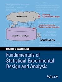
Figure 1.1 is a cartoon view of this process. There is a data cloud, from which information is precipitating. But this information may be fuzzy, indistinct, disorganized, and incomplete. The purpose of statistical analysis is to collect that information and distill it into clear, well-organized INFORMATION. But this process does not work on its own. Intervention is needed. First, if we do some cloud seeding at the start—planning studies and designing experiments—we should increase the amount and quality of precipitating information, and we should facilitate the distillation process. That is, with good planning, it should take less work to extract information from the data. Further, the distillation process needs catalysts—subject-matter knowledge, models, assumptions, and statistical methods. The aim of this text is to provide plans and analysis methods for turning ideas into experiments which yield data that yield information that translates into knowledge and actions based on our improved state of knowledge.
Figure 1.1 Statistics Schematic.
Good experimentation starts with subject-matter knowledge and passion—a strong desire to better understand natural and created phenomena. From this passion flow questions to be answered, questions that can best be posed from a foundation of subject-matter understanding. Statistics provides the tools and framework (i) for translating these questions into experiments and (ii) for interpreting the resulting data. We need to run experiments that are efficient and that are capable of answering questions; we need statistical methods to discover and characterize relationships in the experimental data and to answer whether apparent relationships are real or could easily be random. We need subject-matter knowledge and context to interpret and act on the relationships that are found in the experiments. Subject-matter knowledge and statistical methods need to be intertwined to be most effective in conducting experiments and learning from the resulting data.
Communication
Learning has to be communicated. As mentioned in the Preface, Archie Bunker, of the All in the Family TV show (check your cable TV listings for reruns), once told his son-in-law (approximately, and with typical inadvertent profundity), “Don’t give me no stastistics (sic), Meathead! I want facts!” What he meant was: talk to me in terms of the subject-matter, not in statistical jargon.
Statistics is inherently collaborative—a team sport. Successful experiments require subject-matter knowledge and passion and the statistical tools to translate that knowledge and passion into useful information. Statisticians tend to be passionate about the methods they can use to extract information from data. That’s what they want to talk about. For the collaborative professional in another field, those methods are only a means to an end: revealing and understanding new facts pertinent to his or her area of interest/passion. The experiment and resulting data advance understanding in that field, so it is essential, as Archie said, that statistical results be communicated in this context, not as “statistics” per se.
Subject-Matter Passion
An example that shows the importance of bringing subject-matter passion to the appreciation and interpretation of data is a case study I call “Charlie Clark and the Car Charts.” The statistics group I managed at Sandia National Laboratories in Albuquerque had a small library, and when we got a new addition, I would route it around to the group so they would be aware of it. One new book I routed dealt with graphical methods. Charlie Clark was both thorough and a car nut. He did more than skim the table of contents—he read the book. One chart he came across was a scatter plot of automobile engine displacement versus body weight. This plot (approximately reproduced in Fig. 1.2) showed a slightly curved positive association—heavier cars have larger engines—and a couple of outlying points. The authors made the statistical points that you could not “see” the relationship between body size and engine size, or the outliers in a table of the data, whereas a plot shows these clearly. Then they commented that the outliers might be unusual cars or mistakes in the data and went on to other topics.
Figure 1.2 Car Data: Engine Size versus Body Weight.
Well, the two outlying cars are more than just unusual to a car nut. They would be special: the outlying points are two cars with unusually large engines for their body weights. They would thus be high-performance autos, so Charlie not only noticed the outliers, he got excited. He wanted one of those cars, so he looked up the source data (provided in the book’s appendices). Alas, they were the Opel and Chevette, which he knew were performance dogs—“econoboxes.” He then went to the original Consumer Reports data source and found that transcription errors had been made between the source data and the text. Sorry, Charlie.
The moral of this story is that Charlie found the true “message” in the data (albeit only a transcription error), which is what statistical analysis is all about, not because he was a better statistician than the authors, but because he had a passionate interest in the subject matter. For more on this theme, see Easterling (2004, 2010). See also Box (1984).
Case Study
Integrated circuits (ICs), the guts of computing and communication technology, are circuits imprinted on tiny silicon chips. In a piece of electronic equipment, these ICs are attached to a board by teensy wires, soldered at each end. Those solder joints have to be strong enough to assure that the connection will not be broken if the equipment is jostled or abused to some extent in use. In other words, the wire bonds have to be reliable.
To assure reliability, producers periodically sample from production and do pull-tests on a chip’s bonds. (These tests are usually done on chips that have failed for other reasons—it’s not good business practice to destroy good product.) The test consists of placing a hook under the wire and then pulling the hook until the wire or wire bond breaks. This test is instrumented so that the force required to break the bond is recorded. A manufacturer or the customer will specify a lower limit on acceptable strength. If too many bonds break below this breaking-strength limit, then that is a sign that the bonding process is not working as designed and adjustments are needed.
Well, a process engineer showed up at Ed Thomas’s office one day with a file of thousands of test results collected over some period of time. (Ed is a statistician at Sandia National Laboratories, Albuquerque, NM.) The engineer wanted Ed to use the data to estimate wire-bond reliability. This reliability would be the probability that a bond strength exceeds its acceptable lower limit. (Although we haven’t discussed “probability” yet, just think in terms of a more familiar situation, such as the SAT scores of high school seniors in 2014. These scores vary and a “probability distribution”—sometimes a “bell-shaped curve”—portrays this variability.) The initial plan was to use the data to estimate a “probability distribution” of bond strength and, from this distribution, estimate the percent of the distribution that exceeded the lower limit (see Fig. 1.3).
Figure 1.3 Bond-Strength Distribution.
The bars are the percentages of bond-strength measurements in specified, adjacent intervals. The blue curve is a “Normal Distribution” fitted to the bond-strength data. The estimated reliability is the percent of the distribution above the lower limit.
But Ed was inquisitive—snoopy (and bright). He noticed that the data file did not just have bond-strength data and chip identification data such as date and lot number. The file also had variables such as “bond technician” and “test operator” associated with each test result. He sorted and plotted the bond-strength data for different bond and test operators and found differences. Bond strength seemed to depend on who did the bonding operation and who did the test! This latter dependence is not a good characteristic of an industrial measurement process. You want measurement process components, both equipment and personnel, to be consistent no matter who is doing the work. If not, wrong decisions can be made that have a substantial economic impact. You also want a manufacturing process to be consistent across all the personnel involved. A problem with the available data, though, was that the person who did the bonding operation was often the same person who did the test operation. From these data, one could not tell what the source of the inconsistency was. It would not make sense to try to estimate reliability at this point: you would have to say (apparent) reliability depends on who did the test. That doesn’t make sense. What was needed was further investigation and process improvement to find the source of the inconsistencies in the data and to improve the production and test processes to eliminate these inconsistencies.
After a series of discussions, the process engineer and Ed came up with the following experiment. They would have three operators each use three different machines to make wire bonds. That is, chips would be bonded to packages using all nine possible combinations of operator and machine. Then the boards for each of these combinations would be randomly divided into three groups, each group then pull-tested by a different test operator. This makes 27 combinations of bond operator, machine, and test operator in the experiment. For each of these combinations, there would be two chips, each with 48 bonds. Thus, the grand total of bond-test results would be 27 × 96 = 2592. This is a large experiment, but the time and cost involved were reasonable. These are the sorts of issues faced and resolved in a collaborative design of an experiment.
Statistical analysis of the data, by methods presented in later chapters, led to these findings:
There were no appreciable differences among bonding machines.
There were substantial differences among both bonding operators and test operators.
A couple of points before we look at the data: (i) It is not surprising to find that machines are more consistent than people. Look around. There’s a lot more variation among your fellow students than there is in the laptops or tablets they use. (ii) Because the experiment was “balanced,” meaning that all combinations of bonding and test operators produced the same number of bond tests, it is now possible to separate the effects of bond operator and test operator in the experiment’s data.
Figure 1.4 shows the average pull strengths for each combination of bond and test operators. These averages are averages across machines, chips, and bonds—total of 288 test results in each average.
Figure 1.4 Average Bond Strengths by Bonding and Pull-Test Operators.
The results in Figure 1.4 have very consistent patterns:
Bond operator B produces consistently stronger bonds.
There are consistent differences among pull-test operators—operator A consistently had the highest average pull strengths; operator B consistently had the lowest.
(Statistical number crunching showed that these patterns could not be attributed to the inherent variability of the production and testing processes; they were “real” differences, not random variation.)
Overall, in Figure 1.4, there is nearly a factor of two between the average pull strength for the best combination of operators and for the worst (9.0 vs. 5.1 g). You do not want your production and measurement systems, machines and people, to be this inconsistent.
With this data-based information in hand, the process engineer has a license to examine the production and testing procedures carefully, along with the technicians involved, and find ways to eliminate these inconsistencies.
(A friend of mine tells his audiences: “Without data you’re just another loudmouth with an opinion!” Another often-used statistical funny: “In God we trust. All others bring data.”)
The focus for process improvement has to be on procedures—not people. We’re not going to fire bond operator C because he produced the weakest bonds. We’re going to find out what these operators are doing differently to cause this disparity. It could be that they are interpreting or remembering possibly unclear process instructions in different ways. That can be fixed.
One specific subsequent finding was that it made a difference in pull-testing if the hook was centered or offset toward one end of the wire or the other. Making the instructions and operation consistent on that part of the process greatly reduced the differences among test operators. (Knowing where to place the hook to best characterize a bond’s strength requires subject-matter knowledge—physics, in this case.) Additional iterations of experimenting and process improvement led to much better consistency in the production and testing procedures.
Summary: The process engineer came to Ed wanting a number—a “reliability.” Ed, ever alert, found evidence that the (observational) data would not support a credible reliability number. Well-designed and well-executed experiments found evidence of production and testing problems, and the process engineer and technicians used these findings and their understanding of the processes to greatly improve those processes. Labor and management were both happy and heaped lavish praise on Ed.
This picture is not Ed, but it could have been. The voice-over of this celebratory scene in an old Microsoft Office commercial told us that “With time running out, he took an impossibly large amount of data and made something incredibly beautiful.” May every person who studies this book become a data hero such as this!
Overview of Text
Chapter 2 describes the basic elements of experimental design: experimental units, treatments, and blocks. (Briefly, “treatments” is statistical terminology for the interventions in a process.) Three principles that determine the precision with which treatment “effects” can be estimated—replication, randomization, and blocking—are defined and discussed.
Chapter 3 addresses the fundamentals of statistical data analysis, starting with my recommended Analysis 1: Plot the Data. In particular, plot the data in a way that illuminates possible relations among the variables in the experiment.
Next come quantitative analyses—number crunching. In my view, the fundamental concept of statistical analysis is a comparison of “the data we got” to a probability distribution of “data we might have gotten” under specified “hypotheses” (generally assumptions about treatment effects). Significance tests and confidence intervals are statistical findings that emerge from these comparisons and help sort out and communicate the facts and the statistics, in Archie Bunker’s formulation. Two two-treatment examples from Box, Hunter, and Hunter (1978, 2005) are the launching pads for a wide-ranging discussion of statistical methods and issues in Chapter 3.
Chapter 4 introduces the family of completely randomized designs for the case of one treatment factor, either quantitative or qualitative. Chapter 5 is about completely randomized designs when the treatments are comprised of combinations of two or more treatment factors.
Chapter 6 introduces the family of randomized block designs and considers various treatment configurations. Chapter 7, titled Other Experimental Designs, addresses designs that are hybrids of completely randomized and randomized block designs or that require extending the principles of experimental design beyond the scope of these design families.
And that’s it. This book is meant to be introductory, not comprehensive. At various points, I point to extensions and special cases of the basic experimental designs and provide references. Formulas are minimized. They can be found in the references or online, if needed. I rely on software, primarily Minitab®, to produce data plots and to crunch the numbers. Other statistical software is available. Microsoft Excel® can be coerced into most of the analyses in this text. I think choice of software now is equivalent to choice of desk calculator 50 years ago: at this point in time, it does not matter that much. My focus is on the experimental design and data analysis processes, including the interplay between statistics and the application, between “friendly, local statisticians” and subject-matter professionals. I try to illustrate data-enhanced collaboration as a way to encourage such approaches to the large and small issues students will face when they leave the university and embark upon a career.
Assignment
Choose one of your areas of passionate interest. Find an article on that topic that illustrates the statistics schematic in Figure 1.1. To the extent possible, identify and discuss what that article tells you about the different elements in that process: data, assumptions, models, methods, subject-matter knowledge, statistical analysis, and information generated and communicated. Evaluate how well you think the article succeeds in producing and communicating useful information. Suggest improvements.
References
Box, G. (1984) The Importance of Practice in the Development of Statistics,
Technometrics
, 26, 1–8.
Box, G., (2006)
Improving Almost Anything: Ideas and Essays
, John Wiley & Sons, Inc., New York.
Box, G., Hunter, W., and Hunter, J. (1978, 2005)
Statistics for Experimenters
, John Wiley & Sons, Inc., New York.
Box, G., Leonard, T., and Wu, C-F. (eds.) (1983)
Scientific Inference, Data Analysis, and Robustness
, pp. 51–84, Academic Press, New York.
Easterling, R. (2004) Teaching Experimental Design,
The American Statistician
, 58, 244–252.
Easterling, R. (2010) Passion-Driven Statistics,
The American Statistician
,
64
, 1–5.
Wikipedia (2015) Dom Pérignon (monk),
http://en.wikipedia.org/wiki/Dom_Pérignon_(monk)
.
2Fundamentals of Experimental Design
Introduction
The experiments dealt within this book are comparative: the purpose of doing the experiments is to compare two or more ways of doing something. In this context, an experimental design defines a suite, or set, of experiments. In this suite of experiments, different experimental units are subjected to different treatments. Responses of the experimental units to the different treatments are measured and compared (statistically analyzed) to assess the extent to which different treatments lead to different responses and to characterize the relationship of responses to treatments. This process will be illustrated numerous ways throughout this book.
Agricultural experimentation, which gave rise to much of the early research on statistical experimental design (see, e.g., Fisher 1947), provides a simple conceptual example. An experimenter wants to compare the crop yield and environmental effects for two different fertilizers. The experimental units are separate plots of land. Some of these plots will be treated with Fertilizer A, and some with Fertilizer B. For example, Fertilizer A may be the currently used fertilizer; Fertilizer B is a newly developed alternative, perhaps one designed to have the same or better crop growth yields but with reduced environmental side effects. Better food production with reduced environmental impact is clearly something a research scientist and the public could be passionate, or at least enthusiastic, about.
In this conceptual experiment, the selection of the plots and the experimental protocol will assure that the fertilizer used on one plot does not bleed onto another. Schedules for the amount and timing of fertilizer application will be set up. Crops will be raised and harvested on each plot, and the crop production and residual soil chemicals will be measured and compared to see if the new fertilizer is performing as designed and is an improvement over the current fertilizer.
This example can be readily translated into other contexts:
Medical experiments in which the experimental units are patients and the treatments evaluated might be a new medication, perhaps at different dosage levels, and a placebo
Industrial experiments in which different product designs or manufacturing processes are to be compared
Market research experiments in which the experimental units are consumers and the treatments are different advertising presentations
Education experiments in which the experimental units are groups of children and the treatments are different teaching materials or methods
The possibilities are endless, which is why experimental design is so important to scientific and societal progress on all fronts.
Note the importance of running comparative experiments. If we applied Fertilizer B to all of our plants in this year’s test, we might get what appear to be very satisfactory yields, perhaps even better than Fertilizer A got in previous years. But we would not know whether Fertilizer A would have gotten comparable yields this year due, say, to especially favorable growing conditions or experimental care compared to previous years. To know whether B is better than A, you have to run experiments in which some experimental units get A, some get B, and all other conditions are as similar as possible.
Moreover, you have to assign A and B to experimental units in a way that does not bias the comparison. And you need to run the experiment with enough experimental units to have an adequate capability to detect a difference between fertilizers, relative to the natural variability of crop yields. For a wide variety of reasons, crop yields on identically sized, similar plots of land, all receiving the same fertilizer treatment, will vary; they won’t be identical. (As car commercials warn about gas mileage: actual results may vary.) The potential average crop-yield differences between plots with Fertilizer A and plots with Fertilizer B have to be evaluated relative to the inherent variability of plots that receive the same fertilizer. In experimental design terminology, to do a fair and effective comparison of Fertilizers A and B, you have to randomize and replicate. These are two principles of experimental design, discussed later in this chapter.
Experimental Structure
The common features of all the preceding examples, the building blocks of a comparative experiment, are:
Experimental units (
eu
s)—the entities that receive an independent application of one of the experiment’s treatments
Treatments—the set of conditions under study
Responses—the measured characteristics used to evaluate the effect of treatments on experimental units
Basically, in conducting an experiment, we apply treatments to experimental units and measure the responses. Then we compare and relate the responses to the treatments. The goal of experimental design is to do this informatively and efficiently. The following sections discuss the above aspects of experimental structures.
Experimental units
The choice of experimental units can be critical to the success of an experiment. In an example given by Box, Hunter, and Hunter (1978, 2005) (which will be abbreviated BHH throughout this book), the purpose of the experiment is to compare two shoe-sole materials for boys’ shoes. The experimental unit could be a boy, and each boy in the experiment would wear a pair of shoes of one material or the other. Or the experimental unit could be a foot, and each boy would wear one shoe of each material. As we shall see, the latter experiment dramatically improves the precision with which the wear quality of the two materials can be compared. Where one foot goes, the other goes also, so the wear conditions experienced (the experimental protocol is for the boys to wear the shoes in their everyday lives for a specific period of time) are very much the same (skateboarding and other one-foot dominant activities not allowed). Such is not the case for different boys with different activities. Some boys are just naturally harder on shoes than other boys. As will be seen in Chapter 3


