Lagrangian Modeling of the Atmosphere E-Book
112,99 €
Mehr erfahren.
- Herausgeber: John Wiley & Sons
- Kategorie: Wissenschaft und neue Technologien
- Serie: Geophysical Monograph Series
- Sprache: Englisch
Published by the American Geophysical Union as part of the Geophysical Monograph Series, Volume 200. Trajectory-based ("Lagrangian") atmospheric transport and dispersion modeling has gained in popularity and sophistication over the previous several decades. It is common practice now for researchers around the world to apply Lagrangian models to a wide spectrum of issues. Lagrangian Modeling of the Atmosphere is a comprehensive volume that includes sections on Lagrangian modeling theory, model applications, and tests against observations. Published by the American Geophysical Union as part of the Geophysical Monograph Series. * Comprehensive coverage of trajectory-based atmospheric dispersion modeling * Important overview of a widely used modeling tool * Sections look at modeling theory, application of models, and tests against observations
Sie lesen das E-Book in den Legimi-Apps auf:
Seitenzahl: 989
Veröffentlichungsjahr: 2013
Ähnliche


CONTENTS
Preface
Lagrangian Modeling of the Atmosphere: An Introduction
1. INTRODUCTION
2. TYPES OF LAGRANGIAN ATMOSPHERIC MODELS
3. ADVANTAGESXS AND DISADVANTAGES OF LAGRANGIAN MODELING
4. METEOROLOGICAL FIELDS TO DRIVE LAGRANGIAN ATMOSPHERIC MODELS
5. APPLICATIONS OF LAGRANGIAN MODELS
Section I: Turbulent Dispersion: Theory and Parameterization
Turbulent Dispersion: Theory and Parameterization—Overview
History of Lagrangian Stochastic Models for Turbulent Dispersion
1. INTRODUCTION
2. EARLY DEVELOPMENT OF THE LAGRANGIAN PERSPECTIVE ON TURBULENT DISPERSION
3. EARLY HEURISTIC COMPUTATIONAL LS MODELS
4. NEW CRITERIA FOR LS MODELS AND THE WELL-MIXED CONDITION
5. APPLICATIONS OF WELL-MIXED LS MODELS
6. OUTSTANDING PROBLEMS AND CRITERIA SUPPLEMENTING THE WELL-MIXED CONDITION
7. CONCLUSION
Lagrangian Particle Modeling of Dispersion in Light Winds
1. INTRODUCTION
2. LAGRANGIAN PARTICLE MODELING
3. MODEL FORMULATION, APPLICATION, AND RESULTS
4. CONCLUSIONS
“Rogue Velocities” in a Lagrangian Stochastic Model for Idealized Inhomogeneous Turbulence
1. INTRODUCTION
2. IDEALIZED 1-D TURBULENCE
3. WELL-MIXED LS MODEL
4. TEST FOR RETENTION OF WELL-MIXED STATE
5. RESULTS
How Can We Satisfy the Well-Mixed Criterion in Highly Inhomogeneous Flows? A Practical Approach
1. INTRODUCTION
2. METHODOLOGY
3. RESULTS
4. SUMMARY/CONCLUSIONS
Section II: Transport in Geophysical Fluids
Transport in Geophysical Fluids—Overview
Out of Flatland: Three-Dimensional Aspects of Lagrangian Transport in Geophysical Fluids
1. INTRODUCTION
2. MATHEMATICAL BACKGROUND
3. NUMERICAL EXPERIMENTS
4. DISCUSSION
A Lagrangian Method for Simulating Geophysical Fluids
1. INTRODUCTION
2. THE LGF METHOD
3. SIMULATIONS OF IDEALIZED FLUIDS
4. LAKE AND OCEAN APPLICATIONS
5. INITIAL ATMOSPHERIC RESULTS
6. SUMMARY AND DISCUSSION
Entropy-Based and Static Stability–Based Lagrangian Model Grids
1. INTRODUCTION
2. NUMERICAL DIFFUSION
3. GRID CONSTRUCTION
4. DISCUSSION AND CONCLUSIONS
APPENDIX A: INTERPOLATION AND NUMERICAL DIFFUSION
Moisture Sources and Large-Scale Dynamics Associated With a Flash Flood Event
1. INTRODUCTION
2. DATA AND METHODOLOGY
3. FLASH FLOOD EVENT IN THE REGION OF LISBON (NOVEMBER 1983)
4. LARGE-SCALE ATMOSPHERIC CONDITIONS ASSOCIATED WITH THE EXTRATROPICAL CYCLONE DEVELOPMENT
5. MOISTURE SOURCES, SINKS, AND TRANSPORT
6. SUMMARY AND CONCLUDING REMARKS
The Association Between the North Atlantic Oscillation and the Interannual Variability of the Tropospheric Transport Pathways in Western Europe
1. INTRODUCTION
2. METHODS AND DATA
3. RESULTS
4. DISCUSSION AND CONCLUSIONS
Section III: Applications of Lagrangian Modeling: Greenhouse Gases
Applications of Lagrangian Modeling: Greenhouse Gases—Overview
Estimating Surface-Air Gas Fluxes by Inverse Dispersion Using a Backward Lagrangian Stochastic Trajectory Model
1. INTRODUCTION
2. THE NICHE FOR INVERSE DISPERSION BY BLS
3. MO-BLS IN UNDISTURBED FLOW
4. INVERSE DISPERSION IN STRONGLY DISTURBED FLOWS: 3D-BLS
5. APPLICATIONS OF MO-BLS
6. CONCLUSION
Linking Carbon Dioxide Variability at Hateruma Station to East Asia Emissions by Bayesian Inversion
1. INTRODUCTION
2. METHODOLOGY
3. RESULTS AND DISCUSSION
4. SUMMARY AND CONCLUSIONS
The Use of a High-Resolution Emission Data Set in a Global Eulerian-Lagrangian Coupled Model
1. INTRODUCTION
2. GELCA MODEL
3. ATMOSPHERIC CO2 DATA
4. EMISSION DATA
5. RESULTS AND DISCUSSION
6. SUMMARY AND CONCLUSION
Toward Assimilation of Observation-Derived Mixing Heights to Improve Atmospheric Tracer Transport Models
1. INTRODUCTION
2. METHODS
3. RESULTS
4. DISCUSSION
5. CONCLUSION
Estimating European Halocarbon Emissions Using Lagrangian Backward Transport Modeling and in Situ Measurements at the Jungfraujoch High-Alpine Site
1. INTRODUCTION
2. QUALITATIVE SOURCE ATTRIBUTION
3. QUANTITATIVE SOURCE ESTIMATION BY INVERSE MODELING
4. CHALLENGES FOR SIMULATING TRANSPORT TO JUNGFRAUJOCH
5. CONCLUSIONS
Section IV: Atmospheric Chemistry
Atmospheric Chemistry in Lagrangian Models—Overview
1. INTRODUCTION
2. CHEMICAL BOX MODELS
3. PLUME MODELS
4. DOMAIN-FILLING APPROACHES AND LAGRANGIAN CHEMISTRY TRANSPORT MODELS
5. OUTLOOK
Global-Scale Tropospheric Lagrangian Particle Models With Linear Chemistry
1. INTRODUCTION
2. METHODS
3. RESULTS AND DISCUSSION
4. CONCLUSIONS
Quantitative Attribution of Processes Affecting Atmospheric Chemical Concentrations by Combining a Time-Reversed Lagrangian Particle Dispersion Model and a Regression Approach
1. INTRODUCTION
2. APPLICATION OF FRAMEWORK: METHANESULFONIC ACID IN THE ARCTIC
3. METHODOLOGY
4. FLUXES
5. DEPOSITION
6. REACTIONS AND INITIAL CONCENTRATIONS
7. MODEL SYNTHESIS
8. INTERPRETATION OF REGRESSION RESULTS
9. RESULTS OF MSA ANALYSIS
10. DISCUSSION
Section V: Operational/Emergency Modeling
Operational Emergency Preparedness Modeling—Overview
Operational Volcanic Ash Cloud Modeling: Discussion on Model Inputs, Products, and the Application of Real-Time Probabilistic Forecasting
1. INTRODUCTION
2. VOLCANIC ASH DISPERSION MODELING
3. MODEL INPUTS
4. SITUATIONAL AWARENESS BEFORE EVENT OCCURS
5. REAL-TIME ERUPTION MODEL SIMULATIONS ONCE EVENT OCCURS
6. MODEL TO MODEL COMPARISONS: REAL TIME AND POSTEVENT
7. MODEL TO SATELLITE DATA COMPARISONS
8. THE USE OF PROBABILISTIC AND ENSEMBLE ASH MODELING
9. CONCLUSIONS/DISCUSSION
A Bayesian Method to Rank Different Model Forecasts of the Same Volcanic Ash Cloud
1. INTRODUCTION
2. COMMON CHARACTERISTICS OF VOLCANIC ASH CLOUDS
3. STATISTICAL INFERENCE OF TRANSPORT MODELS
4. MODEL COMPARISON FOR 5–7 MAY 2010 ERUPTION OF EYJAFJALLAJÖKULL VOLCANO
5. DISCUSSION
6. CONCLUSIONS
Review and Validation of MicroSpray, a Lagrangian Particle Model of Turbulent Dispersion
1. INTRODUCTION
2. MICROSPRAY DESCRIPTION
3. VALIDATION VERSUS EXPERIMENTS
4. CONCLUSIONS
Lagrangian Models for Nuclear Studies: Examples and Applications
1. INTRODUCTION
2. PRESENTATION OF MODELS
3. APPLICATIONS
4. CONCLUDING REMARKS
AGU Category Index
Geophysical Monograph Series
Published under the aegis of the AGU Books Board
Kenneth R. Minschwaner, Chair; Gray E. Bebout, Kenneth H. Brink, Jiasong Fang, Ralf R. Haese, Yonggang Liu, W. Berry Lyons, Laurent Montési, Nancy N. Rabalais, Todd C. Rasmussen, A. Surjalal Sharma, David E. Siskind, Rigobert Tibi, and Peter E. van Keken, members.
Library of Congress Cataloging-in-Publication Data
Lagrangian modeling of the atmosphere / John Lin, Dominik Brunner, Christoph Gerbig, Andreas Stohl, Ashok Luhar, and Peter Webley, editors.
pages cm. – (Geophysical monograph, ISSN 0065-8448 ; 200)
Includes bibliographical references and index.
ISBN 978-0-87590-490-0 (alk. paper)
1. Atmosphere–Mathematical models. 2. Lagrangian functions. I. Lin, John, 1975- editor of compilation.
QC874.3.L34 2012
551.501’51539–dc23
2012041203
ISBN: 978-0-87590-490-0
ISSN: 0065-8448
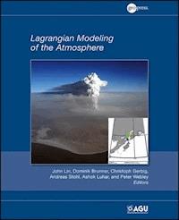
Cover Image: Ash plume from Augustine Volcano on 30 January 2006 during its eruptive stage. Photograph of the plume at 13:09 AKST (22:09 UTC). Photograph credit: Game McGimsey. Image courtesy of Alaska Volcano Observatory/United States Geological Survey. (inset) PUFF volcanic ash Lagrangian Dispersion Particle Model (LDPM) at 22:09 UTC with ash particles indicated by altitude above sea level. Graph courtesy of Peter Webley, Geophysical Institute, University of Alaska Fairbanks.
Copyright 2012 by the American Geophysical Union
2000 Florida Avenue, N.W.
Washington, DC 20009
Figures, tables and short excerpts may be reprinted in scientific books and journals if the source is properly cited.
Authorization to photocopy items for internal or personal use, or the internal or personal use of specific clients, is granted by the American Geophysical Union for libraries and other users registered with the Copyright Clearance Center (CCC). This consent does not extend to other kinds of copying, such as copying for creating new collective works or for resale.The reproduction of multiple copies and the use of full articles or the use of extracts, including figures and tables, for commercial purposes requires permission from the American Geophysical Union. Geopress is an imprint of the American Geophysical Union.
PREFACE
Lagrangian modeling, particularly in the form of mean wind trajectories, has a long tradition in the atmospheric sciences as well as other fields of geosciences, such as oceanography. However, it has experienced explosive growth in the past few decades, thanks to theoretical advances converging with expanded computational power and increased bandwidth, which enables researchers to access three-dimensional meteorological fields from numerical weather prediction centers with which to drive the models.
As a result, Lagrangian models are playing an increasingly important role in different areas of research. Some examples include hydrometeorology, air quality, greenhouse gases, and emergency responses to volcanic eruptions and nuclear releases.
The AGU Chapman Conference “Advances in Lagrangian Modeling of the Atmosphere” was a unique opportunity for a diverse range of atmospheric researchers engaged in Lagrangian modeling, including theoreticians, developers, users, and observationalists, to congregate in the same room over 5 days in October 2011, surrounded by the beautiful scenery of Grindelwald, Switzerland.
The monograph you are holding was inspired by this Chapman Conference, as the presentations and discussions made abundantly clear the growing sophistication of Lagrangian modeling and the myriad ways in which Lagrangian approaches have been applied to yield insights into a variety of geophysical phenomena. Furthermore, participants recognized the lack of a comprehensive volume summarizing advances in Lagrangian modeling that would help a researcher starting in this field to quickly get up to speed. The few existing books on Lagrangian modeling are more focused on a single technical area or a specific application.
We hope this volume captures many of the advances in this important field and the excitement that was palpable among participants at the meeting. The reader can learn about the theoretical advances and outstanding problems, as well as the many applications in different fields written by their respective experts. It is our wish that this monograph can help graduate students and new researchers “see the forest,” while providing enough description of individual “trees.”
We owe an explanation to our oceanography colleagues. The decision was made during the planning of the Chapman Conference and the monograph to not focus on oceanic applications. This decision was due not to a lack of appreciation for the importance of Lagrangian approaches in oceanography but due to the simple realization that the number of papers would be overwhelming for a single meeting or book. In other words, to do justice to the important applications of Lagrangian models to the oceans, a separate monograph is necessary! That being said, some papers in the current volume explicitly tie together the ocean and the atmosphere through a Lagrangian perspective.
We would like to especially acknowledge the efforts of our fellow editors: Ashok Luhar, Andreas Stohl, and Peter Webley. We are grateful to the invaluable help from Carole Delemont and Stephan Henne during the conference. Financial support for the conference came from the European Science Foundation’s TTORCH Research Networking Programme, the Swiss Academy of Sciences, the Center for Climate Systems Modeling at Swiss Federal Institute of Technology Zurich (ETH Zurich), and the International Foundation High Altitude Research Stations Jungfraujoch and Gornergrat.
Last, but definitely not least, for making this monograph possible, thanks go to AGU Meetings Department staff during the lead-up to the Chapman Conference and to Books Department staff during the preparation of the book.
John C. LinUniversity of Utah
Dominik BrunnerSwiss Federal Laboratories for Materials Science and Technology, Empa
Christoph GerbigMax-Planck-Institut für Biogeochemie
Lagrangian Modeling of the Atmosphre: An Introduction
John C. Lin
Department of Atmospheric Sciences, University of Utah, Salt Lake City, Utah, USA
Trajectory-based (“Lagrangian”) atmospheric transport and dispersion modeling has gained in popularity and sophistication over the previous several decades. The objectives of this paper are twofold: (1) to provide a primer in Lagrangian modeling for readers of this AGU monograph and (2) to set the stage for the more technical and specialized papers that make up the rest of this monograph. Different types of Lagrangian modeling approaches (mean trajectory, box, Gaussian plume, and stochastic particle) are introduced; in addition, the advantages and disadvantages of Lagrangian models are discussed. Finally, linkages are made between the fundamentals of Lagrangian modeling and the content of this monograph.
1. INTRODUCTION
We spend our entire lives bathed in the atmosphere, yet most of us look right through it as if it were not even there. We are reminded of its importance, when we are hit by a cool breeze, soaked by a thunderstorm, choked by smoke, or gasp for breath in exhaustion. We breathe in and out molecules that make up the atmosphere, mostly nitrogen (N2) and oxygen (O2), with small quantities of argon (Ar), water (H2O), carbon dioxide (CO2), and other trace species. As these molecules move, interact, and modify radiant energy, the atmosphere gives rise to the bewildering array of phenomena that we are familiar with: wind, clouds, rainfall, and thunderstorms.
The state of the atmosphere dictates the physical conditions in which society is built, so the pursuit for a deeper understanding of the atmosphere has significant societal implications, in addition to scientific interest [Crutzen and Ramanathan, 2000]. This endeavor takes on added urgency, since humans are now understood to affect the atmosphere in numerous ways [Intergovernmental Panel on Climate Change, 2007], whether increasing the amount of greenhouse gases, altering the climate, or degrading air quality.
A central requirement for understanding the atmosphere is the capacity to model its flow. There are two basic types of reference frames when thinking about the fluid: Lagrangian and Eulerian. Put simply, a Lagrangian perspective follows an “air parcel” (see section 2.1) around, as if one receives information from imaginary sensors, which monitor a fluid parcel’s state as it moves (Figure 1a). This is contrasted with the Eulerian perspective, which is fixed in location and observes changes in fluid properties as the parcels are transported past the location (Figure 1b). The Lagrangian and Eulerian perspectives present complementary information. The Eulerian framework yields changes at a fixed location, which is natural for typical ground-based measurements or when stationary grid cells are adopted in modeling. The Lagrangian perspective follows the air parcel and so is intimately connected to the underlying flow.
The Lagrangian and Eulerian perspectives can be formally interchanged, as often discussed in textbooks on dynamic meteorology [Holton, 1992] and geophysical fluid dynamics [Marshall and Plumb, 2007]. If ψ represents any state variable associated with the air parcel (i.e., velocity, temperature, humidity, or pollutant concentration) and S is a generic source term, then the change in ψ in the Lagrangian reference frame can be written as:
(1a)
where D(…)/Dt represents the rate of change following the air parcel and is a special derivative given several names: the Lagrangian, total, substantial, or material derivative. For instance, if ψ is the temperature, then S denotes the sources/sinks such as diabatic heating or radiative cooling. In the case when ψ represents the velocity u, S stands for forces due to pressure gradients or rotation (such as Coriolis).
Figure 1. Comparison between the (a) Lagrangian and (b) Eulerian perspectives. In the Lagrangian perspective, the observer tracks the state variable(s) ψ of the air parcel as it moves in the atmosphere, while in the Eulerian perspective the observer remains stationary at fixed grid points and tracks the changes in ψ as the air parcel moves by. Note that the air parcel is often found in between grid locations (position is subgrid scale).
The Lagrangian perspective in equation (1a) can be transformed to the Eulerian reference frame with the nonlinear advection term u · ∇ψ:
(1b)
where ∂(…)/∂t represents the rate of change at a fixed position, and ∇ is the spatial gradient operator at the same position.
(2)
Owing to the versatility and numerous advantages of Lagrangian models that will be discussed later, it has been applied to study a large variety of atmospheric phenomena and has grown in popularity and prominence over the previous two decades, with over a hundred papers currently published in the scientific literature every year (Figure 2).
In this introductory paper, the different types of Lagrangian models (section 2) are presented. Advantages and disadvantages of Lagrangian modeling versus its Eulerian counterpart follow in section 3. The particular importance of the underlying driver wind fields is also examined (section 4). Finally, the reader is introduced to the applications of Lagrangian models found within the contents of this monograph (section 5).
2. TYPES OF LAGRANGIAN ATMOSPHERIC MODELS
Different types of Lagrangian models are distinguished by their representations of air parcels. To illustrate the differences between models, let us begin by examining what exactly is an air parcel.
2.1. What Is an Air Parcel?
An air parcel is a concept often employed in atmospheric science. It is a “chunk” of the atmosphere that is large enough to encompass enough molecules to possess well-defined properties such as density, temperature, humidity, and pollutant concentration. On the other hand, it is small enough such that the parcel can be thought of as occupying an infinitesimal location in space. It is similar to the point mass or frictionless billiard ball commonly encountered by students in introductory physics.
Figure 2. Estimates of the number of papers published per year relating to Lagrangian modeling of the atmosphere, between the years 1980 and 2011. “LPDM” papers refer to the number of published works applying or directly contributing to the development of Lagrangian particle dispersion models. “Other” papers show the number of works published on other topics such as mean trajectory modeling, Lagrangian box modeling, Gaussian puff modeling, and Lagrangian coherent structures. The literature search was carried out using Thomson Reuters’s Web of Knowledge (http://apps.webofknowledge.com). While the retrieved papers from the search were manually checked to ensure no spurious papers were included, the possibility remains that a small number of papers may have been omitted. This figure, therefore, represents a lower bound on the number of works published.
The boundaries of an air parcel are fuzzy [Bohren and Albrecht, 1998], and a material surface originally encompassing the initial molecules constantly deforms due to molecular and turbulent diffusion, thereby losing their identities. The fact that individual parcels may lose their identities leads to treatment of many parcels in aggregate: as a box or a puff. Alternatively, numerous parcels can be handled more explicitly: as an ensemble of particles.
2.2. Mean Trajectories, Boxes, Puffs, and Particles
The mean trajectory modeling approach assumes that an air parcel retains its identity, and a single line is sufficient to describe its motion (Figure 3a). As indicated above, however, in order for the parcel to preserve its identity, both molecular and turbulent diffusion have to be neglected. The effect of molecular diffusion is small relative to turbulent diffusion throughout the atmosphere, except within a thin layer of a few centimeters near the ground surface [Stull, 1988]. Thus, the absence of turbulence is the main simplification to be considered in mean trajectories, whose name is based on the fact that the air parcel trajectory is derived by solely considering the mean velocity component and neglecting the turbulent, stochastic component u′ in the Reynolds decomposition of u [Reynolds, 1895]:
(3)
By neglecting turbulence, mean trajectories are the simplest representation and, thus, adopted for the longest time among all of the types of Lagrangian models. Wiin-Nielsen [1959] and Danielsen [1961] provide early examples of mean trajectory models. Such models would be more valid in atmospheric regimes where the flow is laminar or simply less turbulent (e.g., in the stratosphere). However, mean trajectories are poor indicators of average transport within the planetary boundary layer (PBL), where turbulence is strong [Stohl and Wotawa, 1993]. In this region of the atmosphere, an air parcel loses its identity as turbulent mixing and wind shear cause the molecules originally found within the air parcel to be dispersed, and a single trajectory no longer suffices.
Figure 3. Schematic illustrating four types of Lagrangian models: (a) mean trajectories; (b) box models; (c) Gaussian puffs; and (d) Lagrangian particle dispersion models (LPDMs). The gray points or volumes represent air parcels, whether individual ones or in aggregate. Each black circle refers to the center of mass of air parcels at each time step. See main text for details.
Lagrangian box models (Figure 3b) treat numerous parcels in aggregate, as boxes whose volumes are described by the extent of mixing. Movement of the box is simulated by either single or multiple mean wind trajectories, initialized at different locations. Often the box is an atmospheric column whose top is matched to the top of the PBL [Eliassen et al., 1982], in order to capture the effect of strong mixing within the PBL. Examples of Lagrangian box models include the single trajectory-based ELMO-2 model [Strong et al., 2010] and the multiple trajectory-based CiTTYCAT model [Pugh et al., 2012], both of which are applied to simulate atmospheric chemistry. While the multiple trajectory box approach better represents the effects on dispersion of flow deformation than a single trajectory method, the fact that the simulations are still based on mean wind trajectories translates into difficulties in modeling interactions between u′ and wind shear that determine atmospheric dispersion in the lower troposphere. Furthermore, strong wind shear distorts the box and introduces large uncertainties to this approach [Seaman, 2000].
Puff models (Figure 3c) attempt to account for the effects of turbulent dispersion by representing air parcels as puffs that grow in size. The puffs usually take on Gaussian distributions in all three dimensions, following the classical work by G.I. Taylor [Taylor, 1920] describing plume dispersion in stationary, homogeneous turbulence. An example of a Gaussian puff model is CALPUFF [Scire et al., 2000], which has been applied widely for air quality regulatory purposes.
Puff models work best when the turbulence and mean winds remain relatively constant. Puff models have difficulties capturing the interaction between turbulence and shear in mean winds in the PBL and lower troposphere, which distort plumes into non-Gaussian shapes, potentially introducing large biases into the peak concentrations and the plume area, thereby requiring ad hoc parameterizations such as puff splitting [Walcek, 2002]. Moreover, when multiple puffs interact, assumptions about puff merging are necessary.
Particle models (Figure 3d), often referred to as “Lagrangian particle dispersion models” (LPDMs), represent air parcels as particles of equal mass that are transported with random velocities generated by a Markov process [Thomson and Wilson, this volume] as a way to simulate u′ and thus the effects of turbulence. An ensemble of particles is simulated by LPDMs to capture the stochastic effects of turbulence. Owing to the randomness introduced in the particle motion, the numerous particles disperse even when initialized at identical starting locations.
The particles in LPDMs possess special properties: they are small enough such that they “follow all turbulent eddies of the flow without being deformed” but are “large compared to the average distance between molecules” and are “so close in density to the surrounding fluid that neither their gravitational settling nor their buoyancy is significant” [Luhar, this volume].
LPDMs are the most sophisticated and computationally expensive, often tracking many thousands of particles in three dimensions. Whereas a single Gaussian puff sufficed to describe a plume of pollutants, many particles need to be tracked in order to characterize the plume. However, the computational cost is often outweighed by the benefit that LPDMs can bring, since they naturally deal with turbulent dispersion and its interaction with mean wind shear without ad hoc assumptions to split puffs.
Owing to the rapid rise in the availability of computational resources, full 3-D LPDM simulations that were expensive to run just a decade ago are now routinely carried out. Figure 2 shows the increase in papers published employing the LPDM method being particularly marked in the 1990s. Some examples of widely used particle models include FLEXPART [Stohl et al., 2005], HYPACT [Walko et al., 2001], and STILT [Lin et al., 2003]. Some models even have hybrid capabilities that combine puff and particle characteristics. These models include HYSPLIT [Draxler and Hess, 1997], NAME [Jones et al., 2007], and TAPM [Hurley et al., 2005].
Most of the Lagrangian models focusing on tropospheric applications in this monograph are LPDMs. Furthermore, important theoretical advances have been made involving proper treatment of heterogeneous turbulence profiles (i.e., the “well-mixed criterion”) [Thomson, 1987] and handling of boundaries [Wilson and Flesch, 1993].
The focus of the first part in this monograph is on proper formulation of LPDMs. This part includes a historical perspective [Thomson and Wilson, this volume], starting from the classical work by Taylor [1920] and extending all the way to recent advances, almost 100 years later. This part includes a specific case of Lagrangian modeling under low wind speed conditions [Luhar, this volume] and a diagnosis of a potential numerical issue within LPDMs, in which u′ adopts unphysical values (“rogue velocity”) [Wilson, this volume]. A specific parameterization for u′ when turbulence is highly inhomogeneous, within the PBL and at its top, is also found [Lin and Gerbig, this volume].
2.3. Backward-Time Lagrangian Simulations
The trajectories of air parcels can be derived in a time-reversed manner by integrating equation (2) backward in time:
(4)
Because the simulations proceed backward in time from a location of interest (the “receptor”), time-reversed simulations are also referred to as “receptor-oriented” [Gerbig et al., 2003]. Such backward-time Lagrangian simulations can be used to address different questions than their forward-time counterparts (Table 1).
An example of backward Lagrangian simulations long adopted by the atmospheric science community is the “back trajectory” approach, which makes use of backward-time mean wind trajectories [e.g., Blifford and Gillette, 1972; Fox and Ludwick, 1976; Sykes and Hatton, 1976]. Typically, backward-time mean wind trajectories are almost perfectly time reversible: a mean back trajectory followed by a forward run retrieves the same starting position, assuming small enough time steps are adopted to minimize the numerical truncation and interpolation errors.
As discussed in section 2.1, mean wind trajectories are applicable in regions of the atmosphere experiencing minimal turbulence. However, they are subject to significant errors in the lower troposphere, in the vicinity of surface emissions. Yet time-reversed Lagrangian modeling is necessary precisely in the lower troposphere to understand surface emissions. Toward this end, LPDM models that run backward in time have been developed and are increasingly applied over the past decade. Because LPDMs incorporate the stochastic velocity u′, time-reversibility in LPDMs is more difficult to ensure than in mean trajectories. It has been pointed out that time reversibility of LPDM simulations requires attention to the well-mixed criterion, as well as several other physical criteria [Linet al., 2003].
The types of information yielded by backward-time LPDM simulations take on different forms. The “retroplume” [Stohlet al., 2003] refers to the ensemble of Lagrangian particles transported backward in time. From “touchdown velocities” of time-reversed particles, the source region of emissions at micrometeorological scales can be determined [Flesch et al., 1995; Wilson et al., this volume]. The “footprint” of an atmospheric concentration is its sensitivity to a unit emission in upwind source regions and is derived from the locations and times of particles found close to the ground [Lin et al., 2003].
Table 1. Some Examples of Questions That Can Be Addressed by Forward-Time Versus Backward-Time Lagrangian Simulations
Forward
Backward
Where does the air go?
Where does the air come from?
What is the downwind impact of air originating from a location of interest (source)?
What are the upwind influences on the location of interest (receptor)?
Where do tracers get transported?
Where are the source regions of tracers?
How much is the concentration of a passive tracer at downwind locations affected by a unit emission from the source?
How strong is the sensitivity of the receptor to a particular upwind source region?
An example of a research field in which backward-time LPDM models have made widespread contributions is in inverse analyses for diagnosing emissions of trace gases from atmospheric concentrations. Here a common issue is that the number of measurement locations (Nr) is significantly smaller than the number of regions where the emissions need to be solved for (Nu). The backward LPDM runs efficiently to provide the sensitivity of receptor concentrations to upwind source regions (i.e., the Jacobian matrix) [Seibert and Frank, 2004] that is an essential part of the inverse analysis. The interested reader can refer to part 3 of this volume for examples of backward LPDMs applied in the context of inverse analyses. Backward-time LPDM models can also be constructed to simulate sources/sinks of water vapor [Stohl and James, 2004] or chemical transformations of atmospheric compounds [Wen et al., 2012]. Parts 2 and 4 of this monograph contain papers applying backward-time LPDM models to water vapor and atmospheric chemistry, respectively.
3. ADVANTAGES AND DISADVANTAGES OF LAGRANGIAN MODELING
In this section, the advantages and disadvantages of Lagrangian modeling are examined.
3.1. Advantages of Lagrangian Modeling
3.1.1. Availability of trajectory information.
Lagrangian simulations provide trajectory information (either forward or backward in time) that is lacking from Eulerian simulations. The knowledge of air parcel trajectories serves as powerful information to answer scientific questions, as the many papers in this monograph will illustrate.
3.1.2. Physical realism.
The Lagrangian approach is a closer analog to atmospheric flows by simulating air parcels. At its essence, the atmosphere is Lagrangian: air is comprised of molecules, and atmospheric flow consists of molecules being transported. Thus, the Lagrangian approach possesses the potential to better approximate phenomena that exist in atmospheric flows such as mixing [Konopka et al., this volume], transport barriers [Sulman et al., this volume], turbulent eddies [Thomson and Wilson, this volume], and convection [Haertel, this volume].
3.1.3. Capability of describing nondiffusive near-field to sources.
LPDMs, in particular, can capture the physics of turbulent transport in the “near-field” regime close to the sources, where turbulence is nondiffusive (or countergradient). See the work of Thomson and Wilson [this volume] for more details.
3.1.4. Numerical stability.
Owing to the absence of the nonlinear advection term in Eulerian models (equation (1b)) and the resulting linearity of Lagrangian advection (equation (1a)), integration of the Lagrangian equations is numerically stable, even when time steps are taken, which are larger than specified by the Courant-Friedrichs-Lewy criterion [Staniforth and Cote, 1991; Wohltmann and Rex, 2009].
3.1.5. Lack of numerical diffusion.
Eulerian advection is known to smear out scalar gradients due to nonphysical numerical diffusion, whose strength is larger than that of atmospheric diffusion [Shin and Reich, 2009; Smolarkiewicz and Pudykiewicz, 1992]. In contrast, Lagrangian advection is subject to minimal numerical diffusion and preserves scalar distributions where sharp gradients exist in the atmosphere, e.g., the polar vortex [McKenna et al., 2002b]. This enables Lagrangian models to parameterize mixing processes that exhibit stronger fidelity to actual atmospheric mixing [McKenna et al., 2002a; Wohltmann and Rex, 2009; Konopka et al., this volume].
3.1.6. Conservation properties.
The Lagrangian framework is a natural way to express conservation properties: conservation of energy, mass, and momentum follows straightforwardly when one considers the same air parcel and follows its movement. While Eulerian advection schemes may not conserve mass [Brasseur et al., 1999] and may produce spurious negative mixing ratios [Rood, 1987], no such difficulties are encountered when one simply tags a parcel with a tracer concentration and follows it along, as is the case for Lagrangian advection [Henne et al., this volume].
3.1.7. Resolving subgrid scale variability.
The positions of Lagrangian air parcels are not tied to regular grid cells (Figure 1). This means that the air parcels can carry subgrid-scale information, helping to resolving the finer-scale heterogeneity not resolved by Eulerian grid cells [Lin et al., 2003]. This is particularly important in the areas immediately upwind of the receptor site for backward-time models or directly downwind of a source region.
3.2. Disadvantages of Lagrangian Modeling
3.2.1. Computational cost.
Lagrangian models are often computationally cheap to run in comparison to Eulerian models, in large part because they do not solve the atmosphere’s equations of motions, but instead rely on output from Eulerian models (section 4). However, depending on the specific application, the computational cost of Lagrangian models can be significant. This is particularly so for LPDMs that simulate large particle ensembles and adopt small time steps to resolve turbulent velocity fluctuations [Thomson and Wilson, this volume]. With the widespread availability of computational resources, however, the disadvantage associated with computational cost is being overcome. Also, for applications in which the air parcels need not interact with one another, Lagrangian simulations are “embarrassingly parallel” and can be parallelized with minimal effort, in which different parcels can be simulated using separate computational nodes. An example of such a simulation is Lagrangian modeling of a chemically inert trace gas like CO2 [Zeng et al., this volume].
3.2.2. Irregularity of “grids”.
The fact that Lagrangian air parcel positions are not fixed at regular intervals like grid cells in Eulerian models means that the “grid” comprised by the ensemble of trajectories would be irregular, even if the parcels were initialized at regular intervals. This requires an additional procedure of parcel insertion or merging [McKenna et al., 2002a], parcel counting within regular grid cells [Stein et al., 2000; Tinarelli et al., this volume], kernel density estimators [Song et al., 2003], or parcels representing dynamic volume [Haertel, this volume].
3.2.3. Inconsistencies with Eulerian driving meteorological fields.
Most Lagrangian models require gridded output from another Eulerian model to simulate air parcel trajectories. See section 4 for a discussion on this point. The two models can be inconsistent with one another, especially if variables are omitted in the output or interpolated from internal model coordinates to common pressure levels. A new development in Lagrangian modeling is overcoming such inconsistencies by having the Lagrangian model simulate atmospheric dynamics, thereby bypassing the Eulerian model entirely [Alam and Lin, 2008; Haertel, this volume].
4. METEOROLOGICAL FIELDS TO DRIVE LAGRANGIAN ATMOSPHERIC MODELS
The “garbage in, garbage out” principle holds for Lagrangian modeling: the quality of Lagrangian simulations can hardly be enhanced if the input meteorological fields are not improved [e.g., Davis and Dacre, 2009; Kretschmer et al., this volume; Webley and Steensen, this volume]. This means that the driver meteorological fields require as much attention as the Lagrangian model itself.
Other than u, another important quantity provided by the driving meteorology is the mixing height: i.e., the vertical extent and intensity of mixing within the PBL. Applications in trace gas transport are strongly dependent on the mixing height [Gerbig et al., 2008]; yet methods to diagnose these properties from meteorological fields are still unsatisfactory in many cases [Seibert et al., 2000]. This has led to efforts to directly assimilate mixing height observations within the Lagrangian simulations [Kretschmer et al., this volume].
Owing to storage limitations, the Eulerian output is often degraded in temporal (and sometimes in spatial) resolution [Stohl et al., 1995] and interpolated to pressure levels [Hoerling and Sanford, 1993]. One symptom of the degradation in the driving meteorological fields is violation of mass conservation, which has been shown to affect simulated trajectories in a way that forward and backward LPDM simulations yield inconsistent results (nonreversibility) [Lin et al., 2003]. Utilization of assimilated meteorological data from different assimilation cycles, which is required to cover transport periods longer than the forecast period, causes dynamical inconsistencies, with dramatic effects on stratosphere-troposphere exchange fluxes [Stohl et al., 2004]. Owing to the same reason, spurious changes in specific humidity and equivalent potential temperature were observed along Lagrangian trajectories, indicating inconsistencies in the humidity and heat budgets [Stohl et al., 2004].
To minimize inconsistencies between the Eulerian output and the Lagrangian models, efforts have been undertaken to closely couple the two kinds of models, with an eye toward conservation properties [Brioude et al., 2012; Nehrkorn et al., 2010].
5. APPLICATIONS OF LAGRANGIAN MODELS
This monograph includes numerous papers that take advantage of the strengths of Lagrangian models mentioned in section 3 to address geophysical questions of interest.
Part 1 of this volume focuses on the formulation of LPDMs and has already been mentioned above in section 2.1.
Part 2 examines the application of Lagrangian models to study geophysical flows. Trajectories can be used to construct “Lagrangian coherent structures” that reveal transport pathways and mixing characteristics of geophysical flows, both in the atmosphere and the ocean [Sulman et al., this volume]. The geophysical flow can be solved in a Lagrangian frame, taking advantage of its numerical strengths (section 3.1) to build Lagrangian dynamical models of both the atmosphere and the ocean [Haertel, this volume]. Konopka et al. [this volume] examine the issue of numerical diffusion in particular, showing how the strength of numerical diffusion can be controlled explicitly in Lagrangian (irregular) grids to mimic actual atmospheric diffusion. The role of geophysical flows in transporting water, the all-important ingredient of weather and climate, is investigated by Liberato et al. [this volume], who combine Lagrangian investigation of moisture sources and a storm-tracking methodology to study an extreme flood event in Portugal. Orza et al. [this volume] examine the transport pathways in Europe and their association with the North Atlantic Oscillation by adopting a back-trajectory clustering technique.
Part 3 is a compendium of several papers applying Lagrangian models to understand greenhouse gases (GHG). The target species is CO2 in most of the papers, and one paper focuses on halocarbons [Brunner et al., this volume], but the framework and discussion in this part is relevant for most other GHGs (e.g., methane (CH4) or nitrous oxide (N2O)). The framework involves tagging particles in LPDMs with concentrations of GHGs and comparing against measured concentrations to derive regional-scale surface fluxes as part of a formal inverse framework [Brunner et al., this volume; Kretschmer et al., this volume; Oda et al., this volume; Zeng et al., this volume]. The LPDMs are run backward in time, due to the smaller number of GHG observational sites versus the number of source elements (section 2.3). An application of backward-time Lagrangian models to determine micrometeorological (local)-scale emissions is also presented [Wilson et al., this volume].
Part 4 examines species in the atmosphere, which undergo chemical transformations and deposition, unlike many GHGs, which are relatively inert in the atmosphere. An approach is to leverage the myriad advantages for simulating tracer transport in Lagrangian models and combine them with linearized chemistry [Henne et al., this volume]. A related linear approach is to first simulate atmospheric transport backward in time, using a Lagrangian model, and then carry out a regression analysis to solve for coefficients controlling both the rates of chemical mechanisms as well as emission strengths [Benmergui et al., this volume].
Part 5 examines the role of Lagrangian models as a central component of emergency warning systems that predict the transport and dispersion of materials that could pose immediate societal risks, which unfortunately have been amply borne out by two events in recent memory. As demonstrated by the 2010 eruption of Eyjafjallajökull in Iceland, one threat includes volcanic ash [Denlinger et al., this volume; Webley and Steenson, this volume]. Second, the meltdown at Japan’s Fukushima Daiichi nuclear power plant following the 2011 earthquake showed the continuing risk of accidental releases of radioactive species from nuclear sites [Arnold et al., this volume]. This part of the volume also includes an example of a sophisticated LPDM and illustrates its application in simulating accidental releases and urban pollution dispersion [Tinarelli et al., this volume].
In conclusion, the numerous applications discussed throughout this monograph underscore the fact that Lagrangian models play a critical role in helping scientists understand phenomena in the geosciences and assisting human society to grapple with several hazards, either natural or anthropogenic in origin. It is my belief that Lagrangian models will continue to grow in significance as a tool in the researcher’s arsenal (Figure 2) and follow its own “upward trajectory” in sophistication and usefulness.
Acknowledgments. I am grateful to Joshua Benmergui for comments and assistance in preparing Figure 2. Valuable input from fellow editors of this monograph is also acknowledged.
REFERENCES
Alam, J. M., and J. C. Lin (2008), Toward a fully Lagrangian atmospheric modeling system, Mon. Weather Rev., 136(12), 4653–4667.
Arnold, D., et al. (2012), Lagrangian models for nuclear studies: Examples and applications, in Lagrangian Modeling of the Atmosphere, Geophys. Monogr. Ser., doi:10.1029/2012GM001294, this volume.
Benmergui, J., S. Sharma, D. Wen, and J. C. Lin (2012), Quantitative attribution of processes affecting atmospheric chemical concentrations by combining a time-reversed Lagrangian particle dispersion model and a regression approach, in Lagrangian Modeling of the Atmosphere, Geophys. Monogr. Ser., doi:10. 1029/2012GM001254, this volume.
Blifford, I. H., Jr., and D. A. Gillette (1972), The influence of air origin on the chemical composition and size distribution of tropospheric aerosols, Atmos. Environ., 6, 463–480.
Bohren, C. F., and B. A. Albrecht (1998), Atmospheric Thermodynamics, Oxford Univ. Press, New York.
Brasseur, G. P., B. Khattatov, and S. Walters (1999), Modeling, in Atmospheric Chemistry and Global Change, edited by G. P. Brasseur, J. J. Orlando and G. S. Tyndall, pp. 423–462, Oxford Univ. Press, New York.
Brioude, J., W. M. Angevine, S. A. McKeen, and E. Y. Hsie (2012), Numerical uncertainty at mesoscale in a Lagrangian model in complex terrain, Geosci. Model Dev. Discuss., 5, 967–991.
Brunner, D., S. Henne, C. A. Keller, M. K. Vollmer, S. Reimann, and B. Buchmann (2012), Estimating European halocarbon emissions using Lagrangian backward transport modeling and in situ measurements at the Jungfraujoch high-Alpine site, in Lagrangian Modeling of the Atmosphere, Geophys. Monogr. Ser., doi:10.1029/2012GM001258, this volume.
Crutzen, P. J., and V. Ramanathan (2000), The ascent of atmospheric sciences, Science, 290, 299–304.
Danielsen, E. F. (1961), Trajectories: Isobaric, isentropic and actual, J. Meteorol., 18, 479–486.
Davis, L. S., and H. F. Dacre (2009), Can dispersion model predictions be improved by increasing the temporal and spatial resolution of the meteorological input data?, Weather, 64(9), 232–237.
Denlinger, R. P., P. Webley, L. G. Mastin, and H. Schwaiger (2012), A Bayesian method to rank different model forecasts of the same volcanic ash cloud, in Lagrangian Modeling of the Atmosphere, Geophys. Monogr. Ser., doi:10.1029/2012GM001249, this volume.
Draxler, R. R., and G. D. Hess (1997), Description of the HYSPLIT_4 modeling system, Tech. Memo. ERL ARL-224, Natl. Oceanic and Atmos. Admin., Washington, D. C.
Eliassen, A., O. Hov, I. S. A. Isaksen, J. Saltbones, and F. Stordal (1982), A Lagrangian long-range transport model with atmospheric boundary layer chemistry, J. Appl. Meteorol., 21, 1645–1661.
Flesch, T. K., J. D. Wilson, and E. Yee (1995), Backward-time Lagrangian stochastic dispersion models and their application to estimate gaseous emissions, J. Appl. Meteorol., 34, 1320–1332.
Fox, T. X., and J. D. Ludwick (1976), Lead (Pb) concentrations associated with 1000 mb geostrophic back trajectories at Quillayute, Washington, Atmos. Environ., 10, 799–803.
Gerbig, C., J. C. Lin, S. C. Wofsy, B. C. Daube, A. E. Andrews, B. B. Stephens, P. S. Bakwin, and C. A. Grainger (2003), Toward constraining regional-scale fluxes of CO2 with atmospheric observations over a continent: 2. Analysis of COBRA data using a receptor-oriented framework, J. Geophys. Res., 108(D24), 4757, doi:10.1029/2003JD003770.
Gerbig, C., S. Korner, and J. C. Lin (2008), Vertical mixing in atmospheric tracer transport models: Error characterization and propagation, Atmos. Chem. Phys., 8, 591–602.
Haertel, P. (2012), A Lagrangian method for simulating geophysical fluids, in Lagrangian Modeling of the Atmosphere, Geophys. Monogr. Ser., doi:10.1029/2012GM001250, this volume.
Henne, S., C. S. Poberaj, S. Reimann, and D. Brunner (2012), Global-scale tropospheric Lagrangian particle models with linear chemistry, in Lagrangian Modeling of the Atmosphere, Geophys. Monogr. Ser., doi:10.1029/2012GM001247, this volume.
Hoerling, M. P., and L. L. Sanford (1993), On the uncertainty in estimates of atmospheric heating due to data postprocessing, J. Clim., 6, 168–174.
Holton, J. R. (1992), An Introduction to Dynamic Meteorology, Academic Press, San Diego, Calif.
Hurley, P. J., W. L. Physick, and A. K. Luhar (2005), TAPM: A practical approach to prognostic meteorological and air pollution modelling, Environ. Modell. Software, 20, 737–752.
Intergovernmental Panel on Climate Change (2007), ClimateChange 2007: The Physical Science Basis: Contribution of Working Group I to the Fourth Assessment Report of the Intergovernmental Panel on Climate Change, edited by S. Solomon et al., Cambridge Univ. Press, Cambridge, U. K.
Jones, A. R., D. J. Thomson, M. Hort, and B. Devenish (2007), The U.K. Met Office’s next-generation atmospheric dispersion model, NAME III, in Air Pollution Modeling and its Application XVII, edited by C. Borrego and A.-L. Norman, pp. 580–589, Springer, New York.
Konopka, P., F. Ploeger, and R. Müller (2012), Entropy-based and static stability–based Lagrangian grids, in Lagrangian Modeling of the Atmosphere, Geophys. Monogr. Ser., doi:10.1029/2012GM 001253, this volume.
Kretschmer, R., F.-T. Koch, D. G. Feist, G. Biavati, U. Karstens, and C. Gerbig (2012), Toward assimilation of observation-derived mixing heights to improve atmospheric tracer transport models, in Lagrangian Modeling of the Atmosphere, Geophys. Monogr. Ser., doi:10.1029/2012GM001255, this volume.
Liberato, M. L. R., A. M. Ramos, R. M. Trigo, I. F. Trigo, A. M. Durán-Quesada, R. Nieto, and L. Gimeno (2012), Moisture sources and large-scale dynamics associated with a flash flood event, in Lagrangian Modeling of the Atmosphere, Geophys. Monogr. Ser., doi:10.1029/2012GM001244, this volume.
Lin, J. C., and C. Gerbig (2012), How can we satisfy the well-mixed criterion in highly inhomogeneous flows? A practical approach, in Lagrangian Modeling of the Atmosphere, Geophys. Monogr. Ser., doi:10.1029/2012GM001232, this volume.
Lin, J. C., C. Gerbig, S. C. Wofsy, A. E. Andrews, B. C. Daube, K. J. Davis, and C. A. Grainger (2003), A near-field tool for simulating the upstream influence of atmospheric observations: The Stochastic Time-Inverted Lagrangian Transport (STILT) model, J. Geophys. Res., 108(D16), 4493, doi:10.1029/2002JD 003161.
Luhar, A. K. (2012), Lagrangian particle modeling of dispersion in light winds, in Lagrangian Modeling of the Atmosphere, Geophys. Monogr. Ser., doi:10.1029/2012GM001264, this volume.
Marshall, J., and R. A. Plumb (2007), Atmosphere, Ocean, and Climate Dynamics: An Introductory Text, Academic Press, San Diego, Calif.
McKenna, D. S., P. Konopka, J.-U. Grooß, G. Günther, R. Müller, R. Spang, D. Offermann, and Y. Orsolini (2002a), A new Chemical Lagrangian Model of the Stratosphere (CLaMS) 1. Formulation of advection and mixing, J. Geophys. Res., 107(D16), 4309, doi:10.1029/2000JD000114.
McKenna, D. S., J.-U. Grooß, G. Günther, P. Konopka, R. Müller, G. Carver, and Y. Sasano (2002b), A new Chemical Lagrangian Model of the Stratosphere (CLaMS) 2. Formulation of chemistry scheme and initialization, J. Geophys. Res., 107(D15), 4256, doi:10.1029/2000JD000113.
Nehrkorn, T., J. Eluszkiewicz, S. C. Wofsy, J. C. Lin, C. Gerbig, M. Longo, and S. Freitas (2010), Coupled Weather Research and Forecasting–Stochastic Time-Inverted Lagrangian Transport (WRF–STILT) model, Meteorol. Atmos. Phys., 107, 51–64.
Oda, T., et al. (2012), The use of a high-resolution emission data set in a global Eulerian-Lagrangian coupled model, in LagrangianModeling of the Atmosphere, Geophys. Monogr. Ser., doi:10. 1029/2012GM001263, this volume.
Orza, J. A. G., M. Cabello, V. Galiano, A. T. Vermeulen, and A. Stein (2012), The association between the North Atlantic Oscillation and the interannual variability of the tropospheric transport pathways in western Europe, in Lagrangian Modeling of the Atmosphere, Geophys. Monogr. Ser., doi:10.1029/2012GM001315, this volume.
Pugh, T. A. M., et al. (2012), A Lagrangian model of air-mass photochemistry and mixing using a trajectory ensemble: The Cambridge Tropospheric Trajectory model of Chemistry and Transport (CiTTyCAT) version 4.2, Geosci. Model Dev., 5, 193–221.
Reynolds, O. (1895), On the dynamical theory of incompressible viscous fluids and the determination of the criterion, Philos. Trans. R. Soc. London, Ser. A, 186, 123–164.
Rood, R. B. (1987), Numerical advection algorithms and their role in atmospheric transport and chemistry models, Rev. Geophys., 25, 71–100.
Scire, J. S., D. G. Strimaitis, and R. J. Yamartino (2000), A User’s Guide for the CALPUFF Dispersion Model (Version 5.0), 521 pp., Earth Tech, Inc., Concord, Mass.
Seaman, N. L. (2000), Meteorological modeling for air-quality assessments, Atmos. Environ., 34, 2231–2259.
Seibert, P., and A. Frank (2004), Source-receptor matrix calculation with a Lagrangian particle dispersion model in backward mode, Atmos. Chem. Phys., 4, 51–63.
Seibert, P., F. Beyrich, S. E. Gryning, S. Joffre, A. Rasmussen, and P. Tercier (2000), Review and intercomparison of operational methods for the determination of the mixing height, Atmos. Environ., 34, 1001–1027.
Shin, S., and S. Reich (2009), Hamiltonian particle-mesh simulations for a non-hydrostatic vertical slice model, Atmos. Sci. Lett., 10, 233–240.
Smolarkiewicz, P., and J. A. Pudykiewicz (1992), A class of semi-Lagrangian approximations for fluids, J. Atmos. Sci., 49, 2082–2096.
Song, C. K., C. H. Kim, S. H. Lee, and S. U. Park (2003), A 3-D Lagrangian particle dispersion model with photochemical reactions, Atmos. Environ., 37, 4607–4623.
Staniforth, A., and J. Cote (1991), Semi-Lagrangian integration schemes for atmospheric models—A review, Mon. Weather Rev., 119, 2206–2223.
Stein, A. F., D. Lamb, and R. R. Draxler (2000), Incorporation of detailed chemistry into a three-dimensional Lagrangian-Eulerian hybrid model: Application to regional tropospheric ozone, Atmos. Environ., 34, 4361–4372.
Stohl, A. (1998), Computation, accuracy and applications of trajectories—A review and bibliography, Atmos. Environ., 32, 947–966.
Stohl, A., and P. James (2004), A Lagrangian analysis of the atmospheric branch of the global water cycle. Part I: Method description, validation, and demonstration for the August 2002 flooding in central Europe, J. Hydrometeorol., 5, 656–678.
Stohl, A., and G. Wotawa (1993), A method for computing single trajectories representing boundary layer transport, Atmos. Environ., 29, 3235–3238.
Stohl, A., G. Wotawa, P. Seibert, and H. Kromp-Kolb (1995), Interpolation errors in wind fields as a function of spatial and temporal resolution and their impact on different types of kinematic trajectories, J. Appl. Meteorol., 34, 2149–2165.
Stohl, A., C. Forster, S. Eckhardt, N. Spichtinger, H. Huntrieser, J. Heland, H. Schlager, S. Wilhelm, F. Arnold, and O. Cooper (2003), A backward modeling study of intercontinental pollution transport using aircraft measurements, J. Geophys. Res., 108 (D12), 4370, doi:10.1029/2002JD002862.
Stohl, A., O. R. Cooper, and P. James (2004), A cautionary note on the use of meteorological analysis fields for quantifying atmospheric mixing, J. Atmos. Sci., 61(12), 1446–1453.
Stohl, A., C. Forster, A. Frank, P. Seibert, and G. Wotawa (2005), Technical note: The Lagrangian particle dispersion model FLEXPART version 6.2, Atmos. Chem. Phys., 5, 2461–2474.
Strong, J., J. D. Whyatt, C. N. Hewitt, and R. G. Derwent (2010), Development and application of a Lagrangian model to determine the origins of ozone episodes in the UK, Atmos. Environ., 44, 631–641.
Stull, R. B. (1988), An Introduction to Boundary Layer Meteorology, Kluwer Acad., Dordrecht, The Netherlands.
Sulman, M. H. M., H. S. Huntley, B. L. Lipphardt Jr., and A. D. Kirwan Jr. (2012), Out of flatland: Three-dimensional aspects of Lagrangian transport in geophysical fluids, in Lagrangian Modeling of the Atmosphere, Geophys. Monogr. Ser., doi:10.1029/2012GM001279, this volume.
Sykes, R. I., and L. Hatton (1976), Computation of horizontal trajectories based on the surface geostrophic wind, Atmos. Environ., 10, 925–934.
Taylor, G. I. (1920), Diffusion by continuous movements, Proc. London Math. Soc., s2-20(1), 196–212.
Thomson, D. J. (1987), Criteria for the selection of stochastic models of particle trajectories in turbulent flows, J. Fluid Mech., 180, 529–556.
Thomson, D. J., and J. D. Wilson (2012), History of Lagrangian stochastic models for turbulent dispersion, in Lagrangian Modeling of the Atmosphere, Geophys. Monogr. Ser., doi:10.1029/2012GM001238, this volume.
Tinarelli, G., L. Mortarini, S. Trini Castelli, G. Carlino, J. Moussafir, P. Armand, and D. Anfossi (2012), Review and validation of MicroSpray, a Lagrangian particle model of turbulent dispersion, in Lagrangian Modeling of the Atmosphere, Geophys. Monogr. Ser., doi:10.1029/2012GM001242, this volume.
Walcek, C. J. (2002), Effects of wind shear on pollution dispersion, Atmos. Environ., 36, 511–517.
Walko, R. L., C. J. Tremback, and M. J. Bell (2001), HYPACT User’s Guide, 113 pp., ASTER Div., Mission Res. Corp., Fort Collins, Colo.
Webley, P. W., and T. Steensen (2012), Operational volcanic ash modeling: Discussion on model inputs, products, and the application of real-time probabilistic forecasting, in Lagrangian Modeling of the Atmosphere, Geophys. Monogr. Ser., doi:10.1029/2012GM001271, this volume.
Wen, D., J. C. Lin, D. Millet, A. Stein, and R. Draxler (2012), A backward-time stochastic Lagrangian air quality model, Atmos. Environ., 54, 373–386.
Wiin-Nielsen, A. (1959), On the application of trajectory methods in numerical forecasting, Tellus, 11, 180–196.
Wilson, J. D. (2012), “Rogue velocities” in a Lagrangian stochastic model for idealized inhomogeneous turbulence, in Lagrangian Modeling of the Atmosphere, Geophys. Monogr. Ser., doi:10. 1029/2012GM001235, this volume.
Wilson, J. D., and T. K. Flesch (1993), Flow boundaries in random-flight dispersion models: Enforcing the well-mixed condition, J. Appl. Meteorol., 32, 1695–1707.
Wilson, J. D., T. K. Flesch, and B. P. Crenna (2012), Estimating surface-air gas fluxes by inverse dispersion using a backward Lagrangian stochastic trajectory model, in Lagrangian Modeling of the Atmosphere, Geophys. Monogr. Ser., doi:10.1029/2012GM 001269, this volume.
Wohltmann, I., and M. Rex (2009), The Lagrangian chemistry and transport model ATLAS: Validation of advective transport and mixing, Geosci. Model Dev., 2, 153–173.
Zeng, J., H. Nakajima, T. Matsunaga, H. Mukai, K. Hiraki, and Y. Yokota (2012), Linking carbon dioxide variability at Hateruma station to East Asia emissions by Bayesian inversion, in Lagrangian Modeling of the Atmosphere, Geophys. Monogr. Ser., doi:10.1029/2012GM001245, this volume.
J. C. Lin, Department of Atmospheric Sciences, University of Utah, Salt Lake City, UT, USA. ([email protected])


