Track Data-Oriented Maintenance Intervention Limit Determination for Ballasted Light Rail Tracks through Multibody Simulations E-Book

David Camacho Alcocer

• Herausgeber: Books on Demand
• Kategorie: Wissenschaft und neue Technologien
• Serie: Neues verkehrswissenschaftliches Journal
• Sprache: Englisch

Seitenzahl: 218

Veröffentlichungsjahr: 2021

Beschreibung

Light rail trains (LRT) are an important part of public transport but due to perceived high life-cycle costs are not always considered suitable. Life cycle cost reduction might be achieved through a knowledge-based maintenance management rather than just on experience. This work develops limits of maintenance and renewal of LRT systems based on vehicle reactions to the current track quality through measured data, multibody simulations and track geometry indices. An approach based on knowledge would lead to a track condition which allows a safe, comfortable, and under an appropriate maintenance strategy, economically profitable operation.

Leseprobe

Preface

The quality of a railway track describes the correct position and the state of the track body. Both of these aspects change during track use and are particularly susceptible to change immediately after new construction or maintenance activities. In addition to ensuring safety during operation, maintaining a certain level of track quality also has a significant impact on the life cycle costs and availability of the railway infrastructure.

If the quality of the track decreases too much, a disproportionately high amount of maintenance will be required. However, if maintenance is carried out each time a slight drop in the track quality occurs, the number of maintenance interventions and the number of resulting restrictions to operations will increase disproportionately. Therefore, determining the adequate time for maintenance interventions and being able to reliably determine the quality of the track while maintaining normal rail operations are of central importance.

In his dissertation, Mr. Camacho develops a methodical approach to quasi-continuously determine the geometrical quality of the track. His approach takes into account the specific framework conditions for light rail systems so that normally operating vehicles can be used to record measurement data during their operation. Of particular interest in this work is the introduction of the standard BS EN 12299: 2009, a standard normally used for determining traveler comfort, as the basis for modeling the track quality. This new approach demonstrates the complexity of this research topic due to, among other reasons, the classification of different irregularities in the track quality and the filtering out of vehicle-related influences.

The main result of this research is a methodology for recording, evaluating, and interpreting measured values in order to determine the geometrical track quality in relation to vehicle responses with particular respect to minimizing the life cycle costs of light rail system infrastructure by implementing vehicle floor sensors in normal vehicles during normal operations, and by deriving the construction-related track quality based on comfort parameters.

Stuttgart, February 2020

Ullrich Martin

Dedication

To my family, especially my wife and daughters... for a brighter future...

Acknowledgment

First of all, I would like to offer my most grateful thank you to my wife and children. Without their support, sacrifice and effort not a single word in this document would have been possible. Thank you, my loved ones.

Without a doubt, my extended family upholds great merit in keeping the train running. I would specifically like to thank Maria Luigia Scuderi and Winfried Zimmermann, and my own family, my mother, Maria Eugenia Alcocer Maycotte, my father, Mario Camacho Cardona, and my sister Ruth.

Naturally, I would also like to thank Professor Ullrich Martin and Professor Corinna Salander for their great support during these past five and a half years, either through advice or resource provision. My thank you for knowledge and resource support could not be complete without thanking colleagues of both institutes, IEV and IMA. I thank all members for their comments and great discussions. However, there are specific people I would like to mention. From IEV a specially thank to Sebastian Rapp, who reviewed the document; providing important insight and comments. He also pushed me through until this document was submitted. From IMA, I would like to thank Timo Strobel in a very special manner. Timo in fact is greatly responsible for the development of the work through his active involvement, support and discussions.

This acknowledgement would not be complete without including some special people outside my family and academics. Hence, I would also like to thank all my friends and students who through the last five plus years have provided me with, in one way or another, support or advice, especially, Giovacchino Genesio, the Family Volz (esp. Michael and Beatriz), The family Rhein (esp. Dieter and Christine), Hanoch Serebrenik, Gabriela Vega and Maria Luisa Flores.

Last but not least, I would like to thank the Mexican government for the financial support which made it possible to dedicate all this time for the development of this research.

Eidesstattliche Erklärung

Hiermit erkläre ich, dass ich diese Arbeit selbständig verfasst und keine anderen als die von mir angegebenen Quellen und Hilfsmittel verwendet habe.

Stuttgart, den 30.09.2019

David Camacho Alcocer

Table of Contents

List of Figures

List of Tables

Kurzfassung

Abstract

1 Introduction

1.1 Motivation

1.2 Challenges

1.3 Objectives

1.4 Scope of the study

1.5 Methodology

1.6 Structure of the document

2 Track Geometry Quality

2.1 Track quality deterioration and degradation

2.2 Track quality deterioration rate

2.3 Track geometry parameters

2.3.1 Track Irregularities

2.3.2 Track irregularities - wavelength

2.4 European track geometry standards and limits of intervention

2.4.1 Standard EN 13848-1

2.4.2 Standard EN 13848-5

2.4.3 Standard EN 13848-6

2.4.4 Standard EN 14363

2.4.5 Deutsche Bahn AG (DB AG) - RIL 821.1000 and RIL 821.2001.18

2.4.6 Standard EN 12299 (comfort index)

2.4.7 Intervention limits for Light Rail Systems

2.5 Methods to determine track geometry quality

2.5.1 Based on track irregularities - statistical methods

2.5.1.1 Standard deviation and maximum values methods

2.5.1.2 Track Geometry Index (TGI)

2.5.1.3 J-synthetic Coefficient

2.5.1.4 Five parameters of defectiveness (W5)

2.5.1.5 Fractal Analysis

2.5.1.6 MDZ-A Number

2.5.2 Vehicle response analysis (VRA) methods

2.5.2.1 VRA-Method in the Netherlands

2.5.2.2 WGB-Method

2.5.2.3 Transfer Functions (TF)

2.5.2.4 Performance-Based Track Geometry (PBTG)

2.5.2.5 Axle box accelerator performed based indicators

2.5.3 Frequency analysis

2.5.3.1 Power Spectral Density

2.5.3.2 Time-Frequency Analysis

3 Track Data

3.1 Track recording vehicle (TRV)

3.1.1 Chord offset / versine method

3.1.2 Inertial method

3.2 Stuttgart’s Track Recording Vehicle

3.3 Treatment of measured data

3.3.1 Spatial domain treatment

3.3.2 Frequency domain analysis of data

3.4 Use of treated data

3.4.1 Synthetic signals

3.4.2 Synthetic data in simulations

3.4.3 Track Geometry Index (TGI) for LRT systems

4 Track Construction and Maintenance

4.1 Ballasted track construction

4.2 Ballasted track of the system under study

4.3 Maintenance Strategies

4.4 Track segmentation

4.5 Vehicle performance as indicator of track maintenance needs

4.6 Maintenance activities to reestablish the track geometry

4.7 Service life of track components and time of track intervention

5 Determination of an Intervention Limit

5.1 Multibody simulation

5.1.1 Light Rail Vehicle (LRV) model

5.1.2 Excitations in MBS model

5.2 Simulation - vehicle responses

5.3 Limit definition at 50 km/h

5.4 Track geometry index determination

5.5 Track deterioration diagram

5.6 Importance of limits and areas of opportunities

6 Conclusions and Future Work

Glossary

References

Abbreviations

Symbols

Appendix I: Track Irregularities

Appendix II: Conversion between Coordinate Systems

Appendix II.A: Conversion from rail to track coordinate systems

Appendix II.B: Conversion from track to rail coordinate systems

Appendix III: Mean Comfort Calculation

Appendix IV: Track Data Provided and Nomenclature

Appendix V: Synthetic Signal Generation

Appendix VI: Stiffness and Damping Calculations

Appendix VI.A: Calculation of track stiffness

Appendix VI.B: Calculation of track damping

Appendix VII: Vehicle Data

Appendix VIII: Location of Sensors

Appendix IX: Real vs Simulated Vertical Accelerations

Appendix X: Vertical Stress Calculation

Appendix X.A: Calculation of stress for vehicle response based on measured track data and calculation of allowable stress

Appendix X.B: Calculation of stress for vehicle responses based on data with increased magnitudes and comparison to allowable stresses at different depths

Appendix XI: Track Parameter Magnitude Increase

Appendix XII: Magnitude Increase “Fine-Tuning”

Appendix XIII: Flow Charts for Formal Specifications

List of Figures

Figure 1: Share of costs for the Life Cycle of an Urban Railway (own work per (Kochs and Marx 2009))

Figure 2: Central aspects in the infrastructure investment strategy (own work per (Tzanakakis 2013))

Figure 3: Conceptual diagram (higher level) of the study (own work)

Figure 4: Working Definition of Track Quality (own work)

Figure 5: Rail coordinate system (own work per (Andrea Haigermoser 2013))

Figure 6: Track coordinate system (own work per (Andrea Haigermoser 2013))

Figure 7: Wavelengths affecting riding quality (own work)

Figure 8: Example of transferring function of chord measuring (chord division 4m/6m) (own work per (Deutsches Institut für Normung e. V. 2016))

Figure 9: Example of symmetrical chord system (own work)

Figure 10: Example of signal distortion due to chord measurement per (Deutsches Institut für Normung e. V. 2016)

Figure 11: Basicentric axes of the human body (own work per (International Organization for Standardization 1997))

Figure 12: Weighting curve Wb (z direction) and Wd (x,y direction) for mean comfort evaluation (own work per (The British Standards Institution 2009))

Figure 13: Schematics of maintenance intervention levels conceived for LRT systems (own work per (Kochs and Marx 2009))

Figure 14: Fractal plot example pattern of geometry deviation for the track geometry shown per (Hyslip 2002)

Figure 15: Principle of superposition in LIT systems ΣYMISO from individual ΣYSISO per (Luber et al. 2010)

Figure 16: Hamming window applied to signal to reduce spectral leakage (own work)

Figure 17: FFT of signals depicting amplitude’s differences (own work)

Figure 18: PSD smoothing using pwelch function with different number of segments (own work)

Figure 19: PSD standard curves for vertical irregularities per ERRI B176 and FRA (own work)

Figure 20: Chord measuring system - calculation of versine/sagitta per (Lewis 2011)

Figure 21: Transfer function of the GT2 HuDe chord-system (own work)

Figure 22: Stuttgart's Track Recording Vehicle - GT2 HuDe (photos: David Camacho)

Figure 23: Angular measurements of an inertial measuring system (own work)

Figure 24: Chord measuring system configuration per (Andrea Haigermoser 2013)

Figure 25: Chord system measuring principle per (HuDe Mess- & Anlagentechnik GmbH 2011)

Figure 26: Data treatment process for vertical irregularities (own work)

Figure 27: Reconstruction of signals (own work)

Figure 28: Data filtering in forward and reverse directions (own work)

Figure 29: Vertical irregularity of worse day observed against to limits per (The British Standards Institution 2010)

Figure 30: Moving SD of worse vertical track geometry observed against limit per (The British Standards Institution 2010)

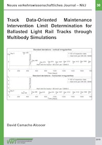
Figure 31: Lateral irregularity of worse day observed against limits (own work)

Figure 32: Moving SD of worse lateral track geometry observed against limit (own work)

Figure 33: Process for the calculation of PSD for vertical irregularities (own work)

Figure 34: PSD of vertical irregularities for the worse, best and latest track geometry quality (own work)

Figure 35: PSD of horizontal irregularities for the worse, best and latest track geometry quality (own work)

Figure 36: PSD of gauge depicting deviation of curves due to lack of filtering (own work)

Figure 37: PSD of gauge irregularities for the worse, best and latest track geometry quality (own work)

Figure 38: PSD of cross level irregularities for the worse, best and latest track geometry quality (own work)

Figure 39: Statistics of signals for Ns 200 (own work)

Figure 40: Signals generated through a Fourier trigonometric function and SIMPACK© (own work)

Figure 41: Vertical vs horizontal SD for tracks 330i and 400i (own work)

Figure 42: Cross section of typical concrete sleeper ballasted track (own work)

Figure 43: Composition of total track modulus C per (Martin et al. 2016; Kerr 2002)

Figure 44: Typical cross section of ballasted track for the system under study per (Benz 2016)

Figure 45: Transition from a current empirical approach to conduct maintenance to a rational-knowledge-based approach per (Tzanakakis 2013)..

Figure 46: Effects of segmentation on a track with known history (own work)

Figure 47: SD development for tr 330 and tr 400 depicting the difference in geometry quality (own work)

Figure 48: Improvement of standard deviations of a track’s parameter due to tamping per (Lichtberger 2005a)

Figure 49: Principles of an integrated track maintenance per (Popovic et al. 2017)

Figure 50: Global and local coordinate systems showing the relationship of two rigid bodies to one another and to a global reference adapted from (Rill and Schaeffer 2010)

Figure 51: Tangential forces and moment developed at the contact patch adapted from (Rill and Schaeffer 2010)

Figure 52: DT8.10 LRT vehicle used to model MBS (photo: author)

Figure 53: DT8.10 SIMPACK© model (own work based on screenshot of MBS model)

Figure 54: Schematic configuration of simulation model adapted from (Strobel etal.)

Figure 55: SIMPACK© model of bogie and suspensions per (Skorsetz et al. September 23 -27)

Figure 56: Comparison of MBS model and real train accelerations (own work)

Figure 57: Accelerations measured by six different sensors spread in passenger cabin according to (The British Standards Institution 2009) (own work)

Figure 58: RMS of signals measured by six different sensors within the passenger cabin per (The British Standards Institution 2009) (own work)

Figure 59: Comfort level of signals measured by six different sensors within the passenger cabin calculated per (The British Standards Institution 2009) (own work)

Figure 60: Process for excitation creation in SIMPACK© based on PSD functions of measured track irregularities (own work)

Figure 61: Comparison of PSD of signal day 320 as measured and as obtained in SIMPACK© (own work)

Figure 62: Comparison of signals generated in SIMPACK© through PSD functions of measured signals vs the signal measured in spatial domain (own work)

Figure 63: Mean comfort index for all days plus day 320 with increased magnitudes (own work)

Figure 64: Mean comfort index development for days after renewal (own work)

Figure 65: SD of vertical (top) and horizontal (bottom) irregularities for track 330 (own work)

Figure 66: Comparison of vertical irregularities produced through double integration versus measured (provided) and simulated vertical irregularities (own work)

Figure 67: Comfort index for synthetic signals displaying higher track irregularities (own work)

Figure 68: Magnitude increase based on track 400 to obtain refined limit values (own work)

Figure 69: Comfort limit for “refined” magnitude increased signals (own work)

Figure 70: PSD of limit values for vertical irregularities (own work)

Figure 71: TGI representation for track 330 for a vehicle riding at 50 km/h (own work)

Figure 72: TGI of track 400 (own work based on (Araji 2018))

Figure 73: Deterioration process of track 330 (own work)

Figure 74: Deterioration process of track 400 (own work per (Araji 2018))...

Figure 75: Track Geometry Parameters (own work per (Deutsches Institut für Normung e. V. 2016))

Figure 76: Mean comfort index NMV calculation process (own work)

Figure 77: Weighting curves Wd and Wb (own work)

Figure 78: Simulated axP and weighted axPWd accelerations in the x-direction (own work)

Figure 79: Simulated ayP and weighted ayPWd accelerations in the y-direction (own work)

Figure 80: Simulated azP and weighted azPWb accelerations in the z-direction (own work)

Figure 81: RMS and 95th percentile of weighted acceleration axPVSWd in the x-direction (own work)

Figure 82: RMS and 95th percentile of weighted acceleration ayP95Wd in the y-direction (own work)

Figure 83: RMS and 95th percentile of weighted acceleration azP95Wb in the z-direction (own work)

Figure 87: Position of sensors in the cabin per (The British Standards Institution 2009) (own work based on image form (Bauer and Theurer 2000; Holzscheiter 2017))

Figure 88: Location of sensors at the axle box of wheels 15 and 16 (own work based on screenshot of MBS model)

Figure 89: Unfiltered accelerations measured in real train at speeds averaging lower than km/h (own work)

Figure 90: Process to treat accelerations measured on real light rail vehicle in Stuttgart (own work)

Figure 91: Comparison between filtered and unfiltered acceleration measured on moving train for a speed average lower than 50 km/h (own work)

Figure 92: Measured acceleration in train at 40 km/h (average speed) vs acceleration in SIMPACK© at 50 km/h (own work)

Figure 93: Measured acceleration in train at 35 km/h (average speed) vs acceleration in SIMPACK© at 50 km/h (own work)

Figure 94: Measured acceleration in train at 44 km/h (average speed) vs acceleration in SIMPACK© at 50 km/h (own work)

Figure 95: Measured acceleration in train at 37 km/h (average speed) vs acceleration in SIMPACK© at 50 km/h (own work)

Figure 96: Measured acceleration in train at 48 km/h (average speed) vs acceleration in SIMPACK© at 50 km/h (own work)

Figure 97: Measured acceleration in train at 34 km/h (average speed) vs acceleration in SIMPACK© at 50 km/h (own work)

Figure 98: Measured acceleration in train at 44 km/h (average speed) vs acceleration in SIMPACK© at 50 km/h (own work)

Figure 99: Measured acceleration in train at 39 km/h (average speed) vs acceleration in SIMPACK© at 50 km/h (own work)

Figure 100: Correction value ks for the Burmeister influence coefficient ks per (Göbel and Lieberenz 2004)

Figure 101: Load influence from the point of maximum load Qmax per TU Darmstadt, Institut für Geotechnik

Figure 102: Stress influence value iz for a circular type loading per TU Darmstadt, Institut für Geotechnik

Figure 103: Normalized values to determine the limit of intervention (own work)

Figure 104: Overview of the research or higher-level processes to conduct the research (own work)

Figure 105: Methodology applied for the development of the research (part 1) - (own work)

Figure 106: Methodology applied for the development of the work (part 2) - (own work)

Figure 107: Level 1.8 - Track data treatment (own work)

Figure 108: Cross Level data treatment (own work)

Figure 109: Gauge data treatment (own work)

Figure 110: Vertical data treatment (own work)

Figure 111: Horizontal data treatment (own work)

Figure 112: Calculation of track Twist (own work)

Figure 113: Calculation of Cross Level in radians (own work)

Figure 114: Calcualtion of Lateral Center line irregularities (own work)

Figure 115: Calculation of PSD of track irregularities (own work)

Figure 116: Calculation of Vertical PSD (own work)

Figure 117: Calculation of Lateral Center line PSD (own work)

Figure 118: Calculation of Cross Level PSD (own work)

Figure 119: Calculation of Gauge PSD (own work)

Figure 120: Determination of irregularities in PSD to use in SIMPACK® (own work)

Figure 121: Simulation of train runs for varying speeds and track geometry to determine vehicle riding characteristics

Figure 122: Simulation of train runs for varying speeds and track geometry to determine vehicle riding characteristics - part 1 (own work)

Figure 123: Simulation of train runs for varying speeds and track geometry to determine vehicle riding characteristics - part 2 (own work)

Figure 124: Simulation of train runs for varying speeds and track geometry to determine vehicle riding characteristics - part 3 (own work)

Figure 125: Conversion of spatial domain signals from SIMPACK© to PSD signals (own work)

Figure 126: Calculation of track geometry index (own work)

List of Tables

Table 1: Wavelength ranges for the assessment of longitudinal level and alignment per (Deutsches Institut für Normung e. V. 2016)

Table 2: Intervention Levels in EN 13848-5 (The British Standards Institution 2010)

Table 3: Track geometry limit values for QN3 level per (The British Standards Institution 2016)

Table 4: Conditions for processing the measuring signals and limit values per (The British Standards Institution 2016)

Table 5: Disturbance / reaction categories per DB regulations per (DB Netz AG: Bautechnik, Leit-, Signal-, u. Telekommunikationstechnik 2004)

Table 6: Limit values at 80 km/h for the different assessment criteria per (DB Netz AG: Bautechnik, Leit-, Signal-, u. Telekommunikationstechnik 2004)

Table 7: Aspects that might be evaluated through the mean comfort index per (The British Standards Institution 2009)

Table 8: SSB’s specified limits of intervention for measured parameters per (Benz 2016)

Table 9: SD limit values for profile and alignment parameters for Alert Limit (AL) per (Deutsches Institut für Normung e. V. 2010)

Table 10: SD values in mm for newly laid track and track needing urgent maintenance per (Research Design and Standards Organisation 1997)

Table 11: Classification of maintenance with TGI per (Talukdar et al. 2006)

Table 12: J Index allowable values at different speeds per (Sadeghi 2010)

Table 13: Quality qualifications of track lines for the five parameter defectiveness (W5) per (Chudzikiewicz et al. 2017)

Table 14: Parameter values for the German PSD standard per (Lei 2017)

Table 15: Parameter values for FRA PSD standard per (Lei 2017)

Table 16: Track data provided by SSB

Table 17: Specifics of filters to treat track irregularity data (own work)

Table 18: Statistics of synthetic signals generated with two different methods

Table 19: TGI values of regular trains and TGI values for LRT system under study

Table 20: Track modulus of different track structural qualities per (Parsons 2012; Powrie and Louis 2016; Martin et al. 2016)

Table 21: Track modulus, damping and stiffness defining the track structural quality of the track (own work)

Table 22: Limits for mean comfort, derrailment coefficient and allowable subgrade stress (own work)

Table 23: Comparison to establish most suitable parameter to determine limits of intervention (own work)

Table 24: Axle -box accelerations to obtain track irregularties from double integration

Table 25: Assesment parameters for riding characteristics per (The British Standards Institution 2016)

Table 26: Factor increase to determine limit values (own work)

Table 27: Vertical and horizontal standard deviation limit values obtained in this study (own work)

Table 28: Track 330 and track 400 maintenance limits

Table 29: Results of acceleration weighting, RMS evaluation and 95th percentile calculation

Table 30: Scale for the mean comfort index NMV per (The British Standards Institution 2009)

Table 31: Track 300 details

Table 32: Track 400 details

Table 33: Calculation of track stiffness for LRT rail 49E1 based on track modulus u

Table 34: Properties of vehicle DT8.10 (Bauer and Theurer 2000)

Table 35: Mass of individual components of the DT8.10 vehicle per (Holzscheiter 2017)

Table 36: Values of suspension components of the DT8.10 per (Holzscheiter 2017)

Table 37: Stifness of the Queranschlag Rollenkranztrager

Table 38: Velocity coefficients per (Göbel and Lieberenz 2004)

Table 39: Subgrade stress σz at 50 and 60 cm and allowable stress σallow at subgrade (own work)

Table 40: Effect of lateral irregularities on comfort level per (Araji 2018)

Table 41: Effect of vertical irregularity on comfort level per (Araji 2018)

Table 42: Horizontal magnitude increase while maintaining the vertical irregularity constant at 6 per (Araji 2018)

Table 43: Increase in vertical irregularity while keeping horizontal irregularities at 3 per (Araji 2018)

Table 44: Increase of magnitudes for all parameters for different values and equal values for all parameters per (Araji 2018)

Table 45: Magnitude increase to obtain limits of intervention that account for vehicle responses (own work)

Table 46: Normalized values using a maximum value not corresponding to the worst limit in the standards (own work)

Kurzfassung

Stadtbahnen (Light rail trains, LRT) bilden einen wichtigen Teil des öffentlichen Personennahverkehrs. Aufgrund der hohen Lebenszykluskosten werden Stadtbahnsysteme jedoch nicht immer als geeignete Lösung betrachtet. Eine Möglichkeit die Lebenszykluskosten zu senken, besteht im Bereich des Instandhaltungsmanagements.

Die Instandhaltung von Stadtbahnstrecken basiert auf Erfahrungswerten der Anlagenverantwortlichen und fokussiert auf die Wartung und die fehlerbehebende Instandhaltung. Dabei wird der aktuelle Streckenzustand nicht immer ausreichend berücksichtigt, wodurch kaum Möglichkeiten zur Kostenoptimierung vorhanden sind. Insbesondere für Stadtbahnsysteme geltende Toleranz-und Grenzwerte für Instandhaltungsmaßnahmen sind bisher weder festgelegt noch ausreichend analysiert, weshalb Grenzen aus Richtlinien der Eisenbahn übernommen werden und dadurch angemessene Intervalle für Wartung- und Instandsetzungsmaßnahmen nicht erreicht werden.

Toleranz- und Grenzwerte für Stadtbahnsysteme sollten auf dem Fahrzeugverhalten basieren, welches wiederum von der aktuellen Gleislagequalität abhängig ist. Dies würde dauerhaft zu einer Gleislage führen, die entweder einen für den Fahrgast komfortablen oder einen für den Infrastrukturbetreiber wirtschaftlichen Betrieb erlaubt.

Der Schwerpunkt dieser Arbeit liegt auf der Bewertung der Gleisgeometrie von Stadtbahnstrecken, für welche, basierend auf der Fahrzeugreaktion, Toleranz- und Grenzwerte für Instandhaltungsmaßnahmen ermittelt werden. Da Daten für Streckenabschnitte in sehr schlechtem Zustand nicht vorhanden waren, werden durch eine sukzessive Erhöhung der Fehleramplituden innerhalb des Frequenzbereichs der gemessenen Gleisgeometrien, künstlich schlechte Gleislagen erzeugt. Die Gleismessdaten werden in eine Mehrkörpersimulationssoftware importiert und die Fahrzeugreaktion bei der Überfahrt von ausgewählten Streckenabschnitten für eine Fahrdauer von fünf Minuten berechnet. Anschließend wird anhand des Fahrkomforts, der Gleisbelastung sowie des Entgleisungskoeffizienten die Fahrzeugreaktion bewertet und auf die Qualität der Gleislage geschlossen.

Zur besseren Darstellung der von der Fahrzeugreaktion abgeleiteten Toleranz- und Grenzwerte für Stadtbahnsysteme wird ein Gleisgeometrieindex eingeführt. Der Gleisgeometrieindex ermöglicht die Darstellung der Verschlechterung der Gleislage und die Einteilung dieser in unterschiedliche Qualitätsstufen. Die Qualitätsstufen helfen Anlagenverantwortlichen, den Zeitpunkt für Instandsetzungsmaßnahmen zielgerichtet festzulegen. Es werden zwei Stadtbahnstrecken detailliert mit der hier entwickelten Methode untersucht. Das Ergebnis deutet darauf hin, dass die in dieser Arbeit betrachteten Strecken zu früh instandgesetzt wurden.

Zukünftige Arbeiten sollen Gleislagefehler durch kontinuierlich gemessene Beschleunigungen am Fahrzeug und im Gleis detektieren. Zusätzlich können Beschleunigungsdaten dann auch für die Beurteilung längerer Streckenabschnitte mit dem hier entwickelten Ansatz genutzt werden.

Abstract

Light rail trains (LRT) form an important part of public transport. However, due to the high life-cycle costs, light rail systems are not always considered a suitable solution. One way to reduce life cycle costs is in the area of maintenance management.

The maintenance of light rail tracks is based on the experience of the infrastructure managers and focuses on preventive and corrective maintenance. The current track condition is not always sufficiently considered, which means there are hardly any possibilities for optimizing costs. In particular, tolerance and limit values for maintenance measures applicable to light rail systems have not yet been defined or adequately analyzed. Instead, limits are taken from the regular railway guidelines, which means that adequate intervals for maintenance and repair measures are not possible.

Tolerances and limits for light rail systems should be based on vehicle reactions, which in turn depends on the current track quality. This would permanently lead to a track condition which allows an operation that is comfortable for the passenger or economically profitable for the infrastructure manager.