Micromechanics with Mathematica E-Book

Seiichi Nomura

• Herausgeber: John Wiley & Sons
• Kategorie: Fachliteratur
• Sprache: Englisch

Seitenzahl: 238

Veröffentlichungsjahr: 2016

Beschreibung

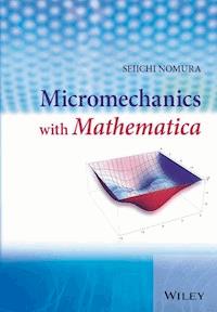
Demonstrates the simplicity and effectiveness of Mathematica as the solution to practical problems in composite materials.

Designed for those who need to learn how micromechanical approaches can help understand the behaviour of bodies with voids, inclusions, defects, this book is perfect for readers without a programming background. Thoroughly introducing the concept of micromechanics, it helps readers assess the deformation of solids at a localized level and analyse a body with microstructures. The author approaches this analysis using the computer algebra system Mathematica, which facilitates complex index manipulations and mathematical expressions accurately.

The book begins by covering the general topics of continuum mechanics such as coordinate transformations, kinematics, stress, constitutive relationship and material symmetry. Mathematica programming is also introduced with accompanying examples. In the second half of the book, an analysis of heterogeneous materials with emphasis on composites is covered.

Takes a practical approach by using Mathematica, one of the most popular programmes for symbolic computation

• Introduces the concept of micromechanics with worked-out examples using Mathematica code for ease of understanding
• Logically begins with the essentials of the topic, such as kinematics and stress, before moving to more advanced areas
• Applications covered include the basics of continuum mechanics, Eshelby's method, analytical and semi-analytical approaches for materials with inclusions (composites) in both infinite and finite matrix media and thermal stresses for a medium with inclusions, all with Mathematica examples
• Features a problem and solution section on the book’s companion website, useful for students new to the programme

Leseprobe

Table of Contents

Cover

Title Page

Copyright

Preface

About the Companion Website

Chapter 1: Coordinate Transformation and Tensors

1.1 Index Notation

1.2 Coordinate Transformations (Cartesian Tensors)

1.3 Definition of Tensors

1.4 Invariance of Tensor Equations

1.5 Quotient Rule

1.6 Exercises

References

Chapter 2: Field Equations

2.1 Concept of Stress

2.2 Strain

2.3 Compatibility Condition

2.4 Constitutive Relation, Isotropy, Anisotropy

2.5 Constitutive Relation for Fluids

2.6 Derivation of Field Equations

2.7 General Coordinate System

2.8 Exercises

References

Chapter 3: Inclusions in Infinite Media

3.1 Eshelby's Solution for an Ellipsoidal Inclusion Problem

3.2 Multilayered Inclusions

3.3 Thermal Stress

3.4 Airy's Stress Function Approach

3.5 Effective Properties

3.6 Exercises

References

Chapter 4: Inclusions in Finite Matrix

4.1 General Approaches for Numerically Solving Boundary Value Problems

4.2 Steady-State Heat Conduction Equations

4.3 Elastic Fields with Bounded Boundaries

4.4 Numerical Examples

4.5 Exercises

References

Appendix A: Introduction to

Mathematica

A.1 Essential Commands/Statements

A.2 Equations

A.3 Differentiation/Integration

A.4 Matrices/Vectors/Tensors

A.5 Functions

A.6 Graphics

A.7 Other Useful Functions

A.8 Programming in

Mathematica

References

Index

End User License Agreement

Pages

ix

x

xi

1

2

3

4

5

6

7

8

9

10

11

12

13

14

15

16

17

18

19

20

21

22

23

24

25

26

27

28

29

30

31

32

33

34

35

36

37

38

39

40

41

42

43

44

45

46

47

48

49

50

51

52

53

54

55

56

57

58

59

60

61

62

63

64

65

66

67

68

69

70

71

72

73

74

75

76

77

78

79

80

81

82

83

84

85

86

87

88

89

90

91

92

93

94

95

96

97

98

99

100

101

102

103

104

105

106

107

108

109

110

111

112

113

114

115

116

117

118

119

120

121

122

123

124

125

126

127

128

129

130

131

132

133

134

135

136

137

138

139

140

141

142

143

144

145

146

147

148

149

150

151

152

153

154

155

156

157

158

159

160

161

162

163

164

165

166

167

168

169

170

171

172

173

174

175

176

177

178

179

180

181

182

183

184

185

186

187

188

189

190

191

192

193

194

195

196

197

198

199

200

201

202

203

204

205

206

207

208

209

210

211

212

213

214

215

216

217

218

219

220

221

222

223

224

225

226

227

228

229

230

231

232

233

234

235

236

237

238

239

240

241

242

243

244

245

246

247

248

249

250

251

252

253

254

255

256

257

258

259

260

261

262

263

264

265

266

267

268

269

270

271

272

273

274

275

Guide

Cover

Table of Contents

Preface

Begin Reading

List of Illustrations

Chapter 1: Coordinate Transformation and Tensors

Figure 1.1 Two-dimensional coordinate transformation

Chapter 2: Field Equations

Figure 2.1 Stress as a black box

Figure 2.2 Traction acting on a plane

Figure 2.3 Surface traction on a curved surface

Figure 2.4 Boundary condition along the line parallel to the axis

Figure 2.5 Boundary condition along the line perpendicular to

Figure 2.6 Principal stresses

Figure 2.7 Mohr's circle

Figure 2.8 Mohr's circle example

Figure 2.9 Strains in one dimension

Figure 2.10 Displacements

Figure 2.11 Rigid rotation by

Figure 2.12 Computations of strains

Figure 2.13 Shear deformation. (a) Pure shear; (b) simple shear

Figure 2.14 2-D orthotropic material.

Figure 2.15 1-D divergence theorem

Figure 2.16 1-D material derivative for a function defined by an integral

Figure 2.17 Curvilinear coordinate system

Figure 2.18 Two-dimensional orthotropic body

Figure 2.19 Gate door

Chapter 3: Inclusions in Infinite Media

Figure 3.1 Inelastic strain

Figure 3.2 Ellipsoidal inclusion

Figure 3.3 Prolate and oblate inclusions

Figure 3.4 Inclusion with

Figure 3.5 Inclusion with with at infinity

Figure 3.6 Inhomogeneity problem with at infinity

Figure 3.7 Stress inside a spherical inclusion

Figure 3.8 Stress inside a cylindrical inclusion ()

Figure 3.9 Multilayered material

Figure 3.10 Two-phase material

Figure 3.11 Three-phase material

Figure 3.12 Four-phase material

Figure 3.13 Thermal stress distribution due to heat source

Figure 3.14 Thermal stress distribution due to heat source

Figure 3.15 Bending of beam subject to shear

Figure 3.16 An infinitely extended body with a hole

Figure 3.17 Three-phase composites

Figure 3.18 Two-dimensional beam

Chapter 4: Inclusions in Finite Matrix

Figure 4.1 Comparison of the first eigenfunction and

Figure 4.2 Comparison of the sixth eigenfunction and

Figure 4.3 Comparison of the first approximate eigenfunction, , and

Figure 4.4 Comparison of the sixth eigenfunction, , and

Figure 4.5 Dirichlet-type boundary condition

Figure 4.6 Neumann-type boundary condition

Figure 4.7 Circular inclusion in a finite medium

Figure 4.8 First base function

Figure 4.10 Third base function

Figure 4.11 Temperature distribution

Figure 4.12 Homogeneous medium

Figure 4.13 Comparison between the Rayleigh–Ritz solution and an FEM solution for the -component of displacement in a homogeneous medium

Figure 4.14 Comparison between the Rayleigh–Ritz solution and an FEM solution for the -component of displacement in a homogeneous medium

Figure 4.15 3-D profile for in the homogeneous medium

Figure 4.16 3-D profile for in the homogeneous medium

Figure 4.17 Contour plot of in the homogeneous medium

Figure 4.18 Contour plot of in the homogeneous medium

Figure 4.19 A medium with a single inclusion

Figure 4.20 Comparison between the Rayleigh–Ritz method and FEM solution for the -component of displacement in the single inclusion problem

Figure 4.21 Comparison between the Rayleigh–Ritz method and FEM solution for the -component of displacement in the single inclusion problem

Figure 4.22 3-D profile of the -component of displacement for the single inclusion problem

Figure 4.23 3-D profile of the

-component of displacement for the single inclusion problem

Figure 4.24 Contour plot of the

-component of displacement for the single inclusion problem

Figure 4.25 Contour plot of the -component of displacement for the single inclusion problem

Figure 4.26 Comparison between the Rayleigh–Ritz method and an FEM solution for the -component of displacement in the single inclusion problem

Figure 4.27 Comparison between the Rayleigh–Ritz method and an FEM solution for the

-component of displacement in the single inclusion problem

Figure 4.28 3-D profile of the

-component of displacement for the single inclusion problem

Figure 4.29 3-D profile of the

-component of displacement for the single inclusion problem

Figure 4.30 Contour plot of the

-component of displacement for the single inclusion problem

Figure 4.31 Contour plot of the -component of displacement for the single inclusion problem

Figure 4.32 Effect of varying inclusion surface areas on the -component of displacement for the single inclusion problem

Figure 4.33 Effect of varying inclusion surface areas on the -component of displacement for the single inclusion problem

Figure 4.34 Effect of varying aspect ratios of the inclusion on the -component of displacement for the single inclusion problem

Figure 4.35 Effect of varying aspect ratios of the constituent phases on the -component of displacement for the single inclusion problem

Figure 4.36 Effect of varying material constants of the constituent phases on the -component of displacement for the single inclusion problem

Figure 4.37 Effect of varying material constants of the constituent phases on the -component of displacement for the single inclusion problem

List of Tables

Chapter 2: Field Equations

Table 2.1 Relation between physical and tensor components

Chapter 3: Inclusions in Infinite Media

Table 3.1 Material properties used in Figure 3.13

Micromechanics with Mathematica

Seiichi Nomura

Department of Mechanical and Aerospace Engineering

The University of Texas at Arlington

Arlington, TX

USA

This edition first published 2016

© 2016 John Wiley & Sons Ltd

Registered office

John Wiley & Sons Ltd, The Atrium, Southern Gate, Chichester, West Sussex, PO19 8SQ, United Kingdom

For details of our global editorial offices, for customer services and for information about how to apply for permission to reuse the copyright material in this book please see our website at www.wiley.com.

The right of the author to be identified as the author of this work has been asserted in accordance with the Copyright, Designs and Patents Act 1988.

All rights reserved. No part of this publication may be reproduced, stored in a retrieval system, or transmitted, in any form or by any means, electronic, mechanical, photocopying, recording or otherwise, except as permitted by the UK Copyright, Designs and Patents Act 1988, without the prior permission of the publisher.

Wiley also publishes its books in a variety of electronic formats. Some content that appears in print may not be available in electronic books.

Designations used by companies to distinguish their products are often claimed as trademarks. All brand names and product names used in this book are trade names, service marks, trademarks or registered trademarks of their respective owners. The publisher is not associated with any product or vendor mentioned in this book.

Limit of Liability/Disclaimer of Warranty: While the publisher and author have used their best efforts in preparing this book, they make no representations or warranties with respect to the accuracy or completeness of the contents of this book and specifically disclaim any implied warranties of merchantability or fitness for a particular purpose. It is sold on the understanding that the publisher is not engaged in rendering professional services and neither the publisher nor the author shall be liable for damages arising herefrom. If professional advice or other expert assistance is required, the services of a competent professional should be sought

Library of Congress Cataloging-in-Publication Data applied for

A catalogue record for this book is available from the British Library.

ISBN: 9781119945031

Preface

Micromechanics is a branch of applied mechanics that began with the celebrated paper of Eshelby published in 1957. It refers to analytical methods for solid mechanics that can describe deformations as functions of such microstructures as voids, cracks, inclusions, and dislocations. Micromechanics is an essential tool for obtaining mechanical fields analytically in modern materials including composite and nanomaterials that did not exist 50 years ago.

There exist a number of well-written books with a similar subject title to this book (micromechanics, continuum mechanics with computer algebra, etc.). However, many of them are written by mathematicians or theoretical physicists that follow the strict style of rigorous formality (theorem, corollary, etc.), which may easily discourage aspiring students without formal background in mathematics and physics yet who want to learn what micromechanics has to offer.

The threshold of micromechanics seems high because many formulas and derivations are based on tensor algebra and analysis that calls for a substantial amount of algebra. Although it is a routine type of work, evaluation of tensorial equations requires tedious manual calculations. This scheme all changed in the 1980s with the emergence of computer algebra systems that made it possible to crunch symbols instead of numbers. It is no longer necessary to spend endless time on algebra manually as symbolically capable software such as Maple and Mathematica can handle complex tensor equations

The aim of this book is to introduce the concept of micromechanics in plain terms without rigorousness yet still maintaining consistency with a target audience of those who want to actually use the result of micromechanics for multiphase/heterogeneous materials, taking advantage of a computer algebra system, Mathematica, rather than those who need formal and rigorous derivations of the equations in micromechanics. The author has been a fan of Mathematica since the 1990s and believes that it is the best tool for handling subjects in micromechanics that require both analytical and numerical computations. Unlike numerically oriented computer languages such as C and Fortran, Mathematica can process both symbols and numerics seamlessly, thus being capable of handling lengthy tensorial manipulations that can release mundane and tedious jobs by human beings. There have been intense debates in user communities about the difference and preference among Mathematica and other numerical software such as MATLAB, all of which are widely used in engineering and scientific communities. The major difference is that software such as MATLAB offers only a limited support for symbolic variables through licensing Maple and is not integrated in the system seamlessly, whereas in Mathematica, there is no distinction between symbolic and numerical variables; more importantly, it is not possible to derive and manipulate formulas employed in this book with MATLAB alone.

One of the unique features in this book is to introduce many examples in micromechanics that can be solved only through computer algebra systems. This includes stress analysis for multiinclusions and the use of the Airy stress function for inclusion problems.

Many of the subjects presented in this book may be classical that may have existed for the past 200 years. Nevertheless, those problems presented in this book would not have been possibly solved analytically had it not been for Mathematica or, for that matter, any computer algebra system, which, the author believes, is the raison d'être of this book.

This book consists of four chapters that cover a variety of topics in micromechanics. Each example problem is accompanied with corresponding Mathematica code. Chapter 1 introduces the basic concept of the coordinate transformations and the properties of Cartesian tensors that are needed to derive equations in continuum mechanics. In Chapter 2, based on the concepts introduced in Chapter 1, the field equations in continuum mechanics are derived. Coordinate transformations in general curvilinear coordinate systems are discussed. Chapter 3 presents a new paradigm for inclusion problems embedded in an infinite matrix. After a brief introduction of the Eshelby method, new analytical approaches to derive the stress fields for an inclusion and concentrically placed inclusions in an infinite matrix are discussed along with their implementations in Mathematica. Chapter 4 is devoted to the inclusion problems where the matrix is finite-sized. The classical Galerkin method is combined with Mathematica to derive the physical and mechanical fields semi-analytically. The Appendix is an introduction to Mathematica that provides sufficient background information in order to understand the Mathematica code presented in this book.

Seiichi NomuraArlington, Texas

About the Companion Website

This book is accompanied by a companion website:

www.wiley.com/go/nomura0615

This website includes:

Listing of Selected Programs

A Solutions Manual

An Exercise Section

Chapter 1Coordinate Transformation and Tensors

To describe the state of the deformation for a deformable body, the coordinate transformation plays an important rule, and the most appropriate way to represent the coordinate transformation is to use tensors. In this chapter, the concept of coordinate transformations and the introduction to tensor algebra in the Cartesian coordinate system are presented along with their implementation in Mathematica. As this book is not meant to be a textbook on continuum mechanics, the readers are referred to some good reference books including Romano et al. (2006) and Fung (1965), among others. Manipulation involving indices requires a considerable amount of algebra work when the expressions become lengthy and complicated. It is not practical to properly handle and evaluate quantities that involve tensor manipulations by conventional scientific/engineering software such as FORTRAN, C, and MATLAB. Software packages capable of handling symbolic manipulations include Mathematica (Wolfram 1999), Maple (Garvan 2001), and others. In this book, Mathematica is exclusively used for implementation and evaluation of derived formulas. A brief introduction to the basic commands in Mathematica is found in the appendix, which should be appropriate to understand and execute the Mathematica code used in this book.

1.1 Index Notation

If one wants to properly express the deformation state of deformable bodies regardless of whether they are solids or fluids, the use of tensor equations is essential. There are several different ways to denote notations of tensors, one of which uses indices and others without using indices at all. In this book, the index notation is exclusively used throughout to avert unnecessary abstraction at the expense of mathematical sophistication.

The following are the main compelling reasons to mandate the use of tensor notations in order to describe the deformation state of bodies correctly.

1.

The principle of physics stipulates that a physically meaningfulobject must be described independent of the frame of references.

1

If the equation for a physically meaningful object changes depending on the coordinate system used, that equation is no longer a correct equation.

2.

Tensor equations can be shown to be invariant under the coordinate transformation. Tensor equations are thus defined as those equations that are unchanged from one coordinate system to another.

Hence, by combining the two aforementioned statements, it can be concluded that only tensor equations can describe the physical objects properly. In other words, if an equation is not in tensorial format, the equation does not represent the object physically.

The index notation, also known as the Einstein notation (Einstein et al. 1916)2 or the summation convention, is the most widely used notation to represent tensor quantities, which will be used in this book. The index notation in the Cartesian coordinate system is summarized as follows:

1.

For mathematical symbols that are referred to quantities in the

,

, and

directions, use subscripts, 1, 2, 3, as in

or

, instead of

or

. The subscripted numbers 1, 2, and 3, refer to the

,

, and

directions, respectively. Obviously, the upper limit of the number is 2 for 2-D and 3 for 3-D.

2.

If there are twice repeated indices in a term of products such as

, the summation with respect to that index (

) is always assumed. For example,

There is no exception to this rule. An expression such as is not allowed as the number of repetitions is 3 instead of 2.

A repeated index is called the dummy index as it does not matter what letter is used, and an unrepeated index is called the free index.3 For example,

all of which represent a summation . An unrepeated index such as (or or ) stands for one of , , or .