Process Design Strategies for Biomass Conversion Systems E-Book

Denny K. S. Ng

• Herausgeber: John Wiley & Sons
• Kategorie: Fachliteratur
• Sprache: Englisch

Seitenzahl: 622

Veröffentlichungsjahr: 2016

Beschreibung

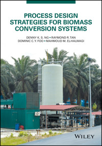
This book covers recent developments in process systems engineering (PSE) for efficient resource use in biomass conversion systems. It provides an overview of process development in biomass conversion systems with focus on biorefineries involving the production and coproduction of fuels, heating, cooling, and chemicals. The scope includes grassroots and retrofitting applications. In order to reach high levels of processing efficiency, it also covers techniques and applications of natural-resource (mass and energy) conservation. Technical, economic, environmental, and social aspects of biorefineries are discussed and reconciled. The assessment scales vary from unit- to process- and life-cycle or supply chain levels.

The chapters are written by leading experts from around the world, and present an integrated set of contributions. Providing a comprehensive, multi-dimensional analysis of various aspects of bioenergy systems, the book is suitable for both academic researchers and energy professionals in industry.

Leseprobe

Table of Contents

Cover

Title Page

List of Contributors

Preface

Acknowledgments

Part 1: Process Design Tools for Biomass Conversion Systems

1 Early-Stage Design and Analysis of Biorefinery Networks

1.1 Introduction

1.2 Framework

1.3 Application: Early-Stage Design and Analysis of a Lignocellulosic Biorefinery

1.4 Conclusion

Nomenclature

References

2 Application of a Hierarchical Approach for the Synthesis of Biorefineries

2.1 Introduction

2.2 Problem Statement

2.3 General Methodology

2.4 Simulation of Flowsheets

2.5 Results and Discussion

2.6 Conclusions

References

3 A Systematic Approach for Synthesis of an Integrated Palm Oil-Based Biorefinery

3.1 Introduction

3.2 Problem Statement

3.3 Problem Formulation

3.4 Case Study

3.5 Conclusions

References

4 Design Strategies for Integration of Biorefinery Concepts at Existing Industrial Process Sites: Case Study of a Biorefinery Producing Ethylene from Lignocellulosic Feedstock as an Intermediate Platform for a Chemical Cluster

4.1 Introduction

4.2 Methodology

4.3 Results

4.4 Conclusions and Discussion

Acknowledgements

Appendix

References

5 Synthesis of Biomass-BasedTri-generation Systems with Variations in Biomass Supply and Energy Demand

5.1 Introduction

5.2 Problem Statement

5.3 Multi-period Optimization Formulation

5.4 Case Study

5.5 Analysis of the Optimization Results

5.6 Conclusion and Future Work

Appendix A

Nomenclature

References

Part 2: Regional Biomass Supply Chains and Risk Management

6 Large-Scale Cultivation of Microalgae for Fuel

6.1 Introduction

6.2 Cultivation

6.3 Harvesting and Dewatering

6.4 Conversion to Products

6.5 Conclusions

Acknowledgments

References

7 Optimal Planning of Sustainable Supply Chains for the Production of

Ambrox

based on

Ageratina jocotepecana

in Mexico

7.1 Introduction

7.2

Ambrox

Supply Chain

7.3 Biomass Cultivation

7.4 Transportation System

7.5

Ambrox

Production

7.6 Bioethanol Production

7.7 Supply Chain Optimization Model

7.8 Case Study

7.9 Conclusions

Acknowledgments

Nomenclature

References

8 Inoperability Input–Output Modeling Approach to Risk Analysis in Biomass Supply Chains

8.1 Introduction

8.2 Input–Output Model

8.3 Inoperability Input–Output Modeling

8.4 Illustrative Example

8.5 Case Study 1

8.6 Case Study 2

8.7 Conclusions

8.8 Further Reading

Appendix A LINGO Code for Illustrative Example

Appendix B LINGO Code for Case Study 1

Appendix C Interval Arithmetic

Appendix D Analytic Hierarchy Process

Nomenclature

References

Part 3: Other Applications of Biomass Conversion Systems

9 Process Systems Engineering Tools for Biomass Polygeneration Systems with Carbon Capture and Reuse

9.1 Introduction

9.2 Production Using Carbon Dioxide

9.3 Process Systems Engineering Tools for Carbon Dioxide Capture and Reuse

9.4 CO

2

Pinch Analysis Tool for Carbon Dioxide Capture and Reuse in Integrated Flowsheet

9.5 Conclusions

References

10 Biomass-Fueled Organic Rankine Cycle-Based Cogeneration System

10.1 Introduction

10.2 Working Fluids for ORC

10.3 Expanders for ORC

10.4 Existing Biomass-Fueled ORC-Based Cogeneration Plants

10.5 Different Configurations of ORC

10.6 Process Description

10.7 Illustrative Example

10.8 Conclusions

References

11 Novel Methodologies for Optimal Product Design from Biomass

11.1 Introduction

11.2 CAMD

11.3 Two-Stage Optimisation Approach for Optimal Product Design from Biomass

11.4 Case Study

11.5 Conclusions

11.6 Future Opportunities

Nomenclature

Appendix

References

12 The Role of Process Integration in Reviewing and Comparing Biorefinery Processing Routes

12.1 Introduction

12.2 Motivating Example

12.3 The Three-Layer Approach

12.4 Production Paths to Xylitol

12.5 Scope for Process and Energy Integration

12.6 Conclusion

Acknowledgment

References

13 Determination of Optimum Condition for the Production of Rice Husk-Derived Bio-oil by Slow Pyrolysis Process

13.1 Introduction

13.2 Experimental Study

13.3 Results and Discussion

13.4 Conclusion

Acknowledgement

References

14 Overview of Safety and Health Assessment for Biofuel Production Technologies

14.1 Introduction

14.2 Inherent Safety in Process Design

14.3 Inherent Occupational Health in Process Design

14.4 Design Paradox

14.5 Introduction to Biofuel Technologies

14.6 Safety Assessment of Biofuel Production Technologies

14.7 Health Assessment of Biofuel Production Technologies

14.8 Proposed Ideas for Future Safety and Health Assessment in Biofuel Production Technologies

14.9 Conclusions

References

Index

End User License Agreement

List of Tables

Chapter 01

Table 1.1 The simplified explanation of each section in SustainPro

Table 1.2 The simplified explanation of each section in LCSoft

Table 1.3 The description of the process intervals presented in Figure 1.7

Table 1.4 The data collection example for Fischer–Tropsch reactor

Table 1.5 Example of the stream table of the Fischer–Tropsch reactor

Table 1.6 Summary table for the data collection (mixing, αi,kk, μi,kk reaction, γi,rr, θreact,rr, waste, SWi,kk, and product, spliti,kk , separation) for thermochemical processing networks (Cheali et al., 2014)

Table 1.7 Summary of the verification results for the Fischer–Tropsch reactor

Table 1.8 The optimization results and comparison. Highlighted in bold are the processing networks for each task

Table 1.9 The top five ranked solutions identified in scenario 2: max. FT-product sales, min. operating cost, and investment cost. Highlighted in bold are the processing networks for each task

Table 1.10 Identified process critical points for the first processing path, regarding the open and closed paths, respectively

Table 1.11 Path flow details on the critical points identified for the first processing path indicated in Table 1.10

Table 1.12 Identified process critical points for the second processing path, regarding the open and closed paths, respectively

Table 1.13 Path flow details on the critical points identified for the second processing path indicated in Table 1.12

Table 1.14 Sustainability metrics for the first and second processing path

Table 1.15 Total carbon footprint for first and second processing path

Table 1.16 Potential environmental impacts for first and second processing path

Chapter 02

Table 2.1 Content of cellulose, hemicellulose, and lignin for some LCM on dry basis (wt%)

Table 2.2 Abbreviations for pretreatments and conversion configurations

Table 2.3 Components for simulations in Aspen Plus

Table 2.4 Properties required for liquid and solid components in Aspen Plus

Table 2.5 Reactions and yield date used in the simulations

Table 2.6 Operating conditions specified into Aspen Plus units

Table 2.7 Specification for separation system used in Aspen Plus

Table 2.8 Effect of using direct recycle on water and ammonia consumption

Table 2.9 Solid content and furfural or acetic acid composition obtained from the simulations

Table 2.10 Comparison of the 16 combination alternatives

Table 2.11 Residence time and dilution rate

Table 2.12 Reactor size for the different configurations

Table 2.13 Annual costs and yearly production

Chapter 03

Table 3.1 Summary of palm-based biomass conversion technologies

Table 3.2 Price of palm-based biomass, product and energy

Table 3.3 Conversion factor for technology pathway

Table 3.4 Energy consumption of each technology

Table 3.5 Economic data of each technology

Table 3.6 Detailed economic analysis of case study

Chapter 04

Table 4.1 Main results of process simulation of the lignocellulosic ethanol production process

Table 4.2 Energy inputs and outputs and overall energy efficiencies at different levels of process integration

Table 4.A.1 Stream data for the lignocellulosic ethanol production plant

Table 4.A.2 Stream data of the ethylene dehydration plant

Table 4.A.3 Stream data with hot and cold utility of the combined ethylene production process

Chapter 05

Table 5.1 Lignocellulosic composition of palm-based biomass and price for Cases 1 and 2

Table 5.2 Cost of utilities

Table 5.3 Fraction of occurrence for low, mid- and high seasons

Table 5.4 Utility demand of a typical POM

Table 5.5 Palm-based biomass availability based on CPO production

Table 5.6 Lignocellulosic composition of palm-based biomass and price for Case 3

Table 5.7 Economic parameters for case study

Table 5.8 Optimization output for Cases 1–3

Table 5.9 Chosen technologies for Cases 1–3

Table 5.10 Available and consumed palm-based biomass for Cases 1–3

Table 5.11 Power distribution for Cases 1–3

Table 5.A.1 Capital costs for each technology based on available design capacity

Table 5.A.2 Conversions for technologies considered

Chapter 06

Table 6.1 Lipid content and productivities of various microalgae species

Table 6.2 Optimal dose and optimal pH range for inorganic and organic flocculants (Uduman et al., 2010 ; Pahl et al., 2013 )

Table 6.3 Fatty acid profiles of some microalgae

Table 6.4 Change in fatty acid profile of Isochrysis sp. as salinity and supply of N are varied

Table 6.5 Carbohydrate composition of selected microalgae

Chapter 07

Table 7.1 Uses of land in each municipality (INEGI, 2010)

Table 7.2 Job generation and cost associated with A. jocotepecana growing

Table 7.3 Transportation costs of raw material, products, and by-products (FIRA, 2007; INEGI, 2010)

Table 7.4 Variable costs of processing plants

Table 7.5 Variable costs associated with the processing plants (SENER, 2006)

Table 7.6 Fixed costs associated with the processing plants (SENER, 2006)

Table 7.7 Jobs generated for Ambrox production

Table 7.8 Production yield

Table 7.9 Values for damages associated with the agriculture of A. jocotepecana

Table 7.10 Values for damages associated with the bioethanol production

Table 7.11 Values for damages associated with the Ambrox production

Table 7.12 Cost comparison (USD)

Table 7.13 Comparison of jobs generated

Table 7.14 Comparison for environmental impact (EI-99/year)

Chapter 08

Table 8.1 Triplet of questions in risk assessment for biomass supply chains

Table 8.2 Triplet of questions in risk management for biomass supply chains

Table 8.3 Flows for a hypothetical two-sector economy (in USD)

Table 8.4 Coefficients of A in case study 1

Table 8.5 Total output (x) and final demand (c) case study 1 (in thousand RM)

Table 8.6 Coefficients of

A

* in case study

Table 8.7 Nomenclature of the 16 economic sectors considered

Table 8.8 Coefficients of A for case study 2

Table 8.9 Updated technical coefficients matrix A due to implementation of 5% biodiesel blend

Table 8.10 Total output and final demand using revised technical coefficients matrix (in thousand PhP)

Table 8.11 Coefficients of the matrix

A

* for a 5% biodiesel blend

Chapter 09

Table 9.1 Biomass ultimate analysis and primary pyrolysis product compositions

Table 9.2 Streams’ compositions and temperature in the flowsheet shown in Figure 9.3

Table 9.3 Basis streams in the key process units for mass and energy balance and capital cost evaluation

Table 9.4 Parameters and calculation of ISBL costs

Table 9.5 Annualised capital cost estimation

Table 9.6 Annualised operating cost estimation

Table 9.7 Product prices and netback

Table 9.8 Mass balance factors for the algae-based biorefinery

Table 9.9 Algae biomass composition (Illman et al. 2000 )

Table 9.10 CO

2

source and demand data extracted from biorefinery flowsheet

Chapter 10

Table 10.1 List of most widely used working fluids in ORC-based plants

Table 10.2 The comparison between various types of expanders used in the ORC-based system

Table 10.3 List of the ORC-based system manufacturers

Table 10.4 Data used for example

Table 10.5 Results, for example, pressure, temperature, and enthalpy for different state points of the ORC (cycle with regeneration)

Table 10.6 Results, for example, main performance parameters

Chapter 11

Table 11.1 Lower and upper bounds for regions with different uncertainty

Table 11.2 Target property ranges for design problem

Table 11.3 Fuzzy membership functions of properties of interest

Table 11.4 List of signatures

Table 11.5 Possible design of bio-based fuel

Table 11.6 Comparison of λ

p

between different designs of bio-based fuel

Table 11.7 Comparison of λ

p

between different designs of bio-based fuel

Table 11.8 Molecular structures for the possible designs of bio-based fuel

Table 11.9 Lignocellulosic composition of EFB

Table 11.10 List of conversion pathways and yield

Table 11.11 Price of products and raw materials

Table 11.12 Capital and operating cost for conversion pathways

Table 11.13 Comparison of results for scenario 1 and 2

Chapter 12

Table 12.1 Parameters imported by user for xylitol component

Table 12.2 Stream properties for the heat integration of the chemical process

Table 12.3 Additional stream for the heat integration

Table 12.4 Hot and cold streams of the biotechnological process

Table 12.5 Properties of stream M1

Table 12.6 Properties of stream M2

Table 12.7 Summarizing results regarding the heat integration in every scenario and case

Chapter 13

Table 13.1 Properties of petroleum fuel

Table 13.2 Properties of RH (wt%)

Table 13.3 Properties of bio-oil produced at different heating rates

Table 13.4 Comparison of bio-oil properties with literatures

Table 13.5 Conversion, gas yield, and residue yield

Chapter 14

Table 14.1 Information availability at different design stages

List of Illustrations

Chapter 01

Figure 1.1 A schematic representation of the development funnel for a project in the processing industries.

Figure 1.2 The integrated business and engineering framework adapted: the dashed boxes indicate the outcome of each step of the workflow

Figure 1.3 The generic process model block.

Figure 1.4 The framework of LCSoft (Kalakul et al., 2014)

Figure 1.5 The superstructure of the biochemical conversion platform of biomass

Figure 1.6 Combined superstructure of two biorefinery conversion platforms: thermochemical (top) and biochemical platform (bottom).

Figure 1.7 Combined superstructure of two biorefinery conversion platforms: thermochemical (top) and biochemical platform (bottom).

Figure 1.8 Process diagram showing mass inlet/outlet, the reaction, and its stoichiometry for the Fischer–Tropsch reactor

Figure 1.9 The simplified process flow diagram of the second best optimal processing path of scenario 2 (as presented in Table 1.9)

Figure 1.10 The simplified process flow diagram of the best optimal processing path of scenario 2 (as presented in Table 1.9)

Chapter 02

Figure 2.1 Case study: bioethanol production based on biochemical platform

Figure 2.2 General methodology

Figure 2.3 Pretreatment flowsheet

Figure 2.4 Pretreatment with direct recycle

Figure 2.5 Conversion configurations based on acid hydrolysis

Figure 2.6 Conversion configurations based on enzymatic hydrolysis

Figure 2.7 Integration between pretreatment and conversion steps

Figure 2.8 Conventional distillation scheme for hydrous ethanol production

Figure 2.9 A summary of results from the methodology application

Figure 2.10 Energy cost for pretreatment options

Figure 2.11 Energy cost for pretreatment with direct recycle

Figure 2.12 Combinations among pretreatment and conversion configurations

Figure 2.13 Energy cost including a conventional distillation step

Chapter 03

Figure 3.1 Global palm oil production 2008/2009 to 2012/2013 (USDA, 2014)

Figure 3.2 Schematic diagram of palm oil mill.

Figure 3.3 Generic superstructure

Figure 3.4 Superstructure of an integrated POB and POM with CHP

Figure 3.5 Optimal configuration of an integrated POB and POM with CHP

Chapter 04

Figure 4.1 Overview of biomass conversion processes and potential products.

Figure 4.2 Material and energy flows across the chemical cluster in Stenungsund (Jönsson et al., 2012 )

Figure 4.3 Overview of biomass-to-ethylene production routes: different biomass conversion technologies to produce ethylene from biomass.

Figure 4.4 Illustration of the heat integration approach. Upper left: base case with no integration between ethanol and ethylene process. Upper right: heat and material integration between the two processes. Lower: heat and material integration and design of a utility system to enable site-wide heat integration

Figure 4.5 Overview of bioethanol production process from lignocellulosic feedstock. Data included shows the process parameters used for process simulation (Stenberg et al., 1998 ; Wooley et al., 1999 ; Aden et al., 2002 ; Galbe & Zacchi, 2002 ; Söderström et al., 2003 ; National Renewable Energy Laboratory, 2004 ; Söderström et al., 2004 ; Sassner et al., 2008 ; Fornell & Berntsson, 2009 )

Figure 4.6 Overview of the ethanol dehydration to ethylene process configuration. Data included shows the process parameters used for process simulation (Stauffer & Kranich, 1962 ; Barrocas et al., 1980 ; Kochar et al., 1981 ; Chematur, 2010 ; Huang, 2010 )

Figure 4.7 GCC of the ethanol production process from lignocellulosic biomass; direct stream injection of 51 MW in the pretreatment steps is considered a process requirement and therefore not included

Figure 4.8 GCC of the ethanol dehydration process; direct steam injection of 25 MW steam to the ethylene reactor is considered a process requirement and therefore not included

Figure 4.9 Background/foreground analysis of the ethanol production and ethanol dehydration process; direct delivery of ethanol between the processes is accounted for in the stream data

Figure 4.10 Total site profile curves of the biorefinery, introducing a utility system with two steam levels (8.8 bar(g), 2 bar(g)): a hot water circuit and direct flue gas heating

Figure 4.11 Total site composite curves of the biomass-to-ethylene plant

Figure 4.12 GCC representing the transfer of heat from hot process streams to an improved utility system in the chemical cluster. Used to determine the amount of additional excess heat possible to deliver to the biorefinery (Hackl et al., 2011 )

Chapter 05

Figure 5.1 Generic representation of superstructure for scenarios.

Figure 5.2 Generic representation of scenarios.

Figure 5.3 Block diagram for case study.

Figure 5.4 Normalized production for POM.

Figure 5.5 Total CPO production in Malaysia for 2013 (Board, 2015).

Figure 5.6 Superstructure for palm BTS

Figure 5.7 Optimal configuration of palm BTS for Case 1 (of maximum economic performance)

Figure 5.8 Optimal configuration of palm BTS for Case 2 (with limit on capital investment)

Figure 5.9 Optimal configuration of palm BTS for Case 3 (with different biomass quality)

Chapter 06

Figure 6.1 An overall framework showing major operations for obtaining fuels from microalgae.

Figure 6.2 Examples of two aquatic microorganisms used for biomass growth: (a) prokaryotic cyanobacteria Spirulina (Simon, 1994) (Photo taken by Joan Simon / CC-BY-SA-2.5). and (b) eukaryotic microalgae Haematococcus (Taka, 2006) (Photo taken by Taka.)

Figure 6.3 Raceway pond

Figure 6.4 Tubular photobioreactor (IGV Biotech, 2013). Photo taken by IGV Biotech.

Figure 6.5 Dunaliella salina farms located in Hutt Lagoon, Australia (Orchard, 2009). The ponds are pink due to the beta-carotene produced by the microalgae. Photo taken by Samuel Orchard.

Figure 6.6 A simplified biodiesel production process.

Figure 6.7 Biodiesels from different sources vary greatly in clarity and color.

Figure 6.8 A possible process flow diagram for utilization of microalgal biomass.

Figure 6.9 A possible process flow diagram for the production of ammonia from cyanobacteria.

Chapter 07

Figure 7.1 (−)-8α-12-Epoxy-13,14,15,16-tetranorlabdane “Ambrox.”

Figure 7.2 Chemical cyclization to obtain Ambrox from tetranorlabdanodiol.

Figure 7.3 Proposed superstructure for the supply chain of Ambrox from A. jocotepecana.

Figure 7.4 Location of the considered municipalities in Michoacán, Mexico (INEGI, 2010)

Figure 7.5 Location of municipalities (preprocessing plants) and Morelia City (central processing plant) in the Michoacán state map (INEGI, 2010)

Figure 7.6 Steps for Ambrox processing.

Figure 7.7 Eco-indicator 99 methodology

Figure 7.8 Pareto curve between the profit and environmental impact.

Figure 7.9 Necessary land for A. jocotepecana cultivation in Quiroga.

Figure 7.10 Results for maximizing the net present value.

Chapter 08

Figure 8.1 Flow of goods, resources, and wastes in a hypothetical three-sector economy

Figure 8.2 Flow of goods in a hypothetical two-sector economy (in USD)

Figure 8.3 Sector inoperability levels in case study 1

Figure 8.4 Sector economic losses in case study 1

Figure 8.5 Sector inoperability levels in case study 2

Figure 8.6 Sector economic losses in case study 2

Chapter 09

Figure 9.1 Structure of bisphenol A polycarbonate

Figure 9.2 Synthesis of poly(propylene carbonate)

Figure 9.3 Conceptual process flowsheet for carbon dioxide capture in Sabatier’s reaction and by adsorbent. The shaded texts indicate products for export to the market

Figure 9.4 Potential CO

2

sources and demands in a biorefinery

Figure 9.5 Methodology for CO

2

integration in a biorefinery.

Figure 9.6 (a) CO

2

purity profile formed by source composite curve (SCC) and demand composite curve (DCC). The areas enclosed between the composite curves correspond to the net CO

2

flow rate shown as horizontal segments in the corresponding (b) CO

2

surplus diagram.

Figure 9.7 (a) The change in flow rate displaces the SCC producing a (b) shift in the surplus diagram until pinched with the y-axis.

Figure 9.8 Algae-based biorefinery process flowsheet. Mass flow rates are in kg h

−1

and energy in MJ h

−1

. The percentage CO

2

purity on mass basis is shown

Figure 9.9 (a) Purity profile showing the demand composite curve (DCC) and the source composite curve (SCC) and (b) surplus diagram for the case study

Figure 9.10 (a) Purity profile and (b) surplus diagram as in the initial network and pinched after the introduction of purification unit

Figure 9.11 (a) Purity profile and (b) surplus diagram pinched after the introduction of purification unit and after reducing the amount of imported flue gas

Figure 9.12 Integrated CO

2

exchange network design for the case study. Flow rates in kg h

−1

and purities in mass percentage

Chapter 10

Figure 10.1 Typical saturation curves on T–s diagram for (a) a dry fluid, (b) an isentropic fluid, and (c) a wet fluid.

Figure 10.2 Schematic diagram of an ORC: (a) flow diagram of a basic ORC and (b) T–s diagram of a basic ORC working with a dry fluid

Figure 10.3 Schematic diagram of an ORC: (a) flow diagram of an ORC incorporating regeneration and (b) flow diagram of an ORC incorporating turbine bleeding

Figure 10.4 Schematic diagram of an ORC: (a) flow diagram of an ORC incorporating turbine bleeding and regeneration and (b) T–s diagram of an ORC incorporating turbine bleeding and regeneration working with a dry fluid.

Figure 10.5 Typical flow diagram of a biomass-fueled organic Rankine cycle-based cogeneration system

Chapter 11

Figure 11.1 Property prediction by using QSPR model.

Figure 11.2 Two-stage optimisation approach to produce optimal product from biomass

Figure 11.3 Procedure for solving a multi-objective chemical product design problem

Figure 11.4 Fuzzy membership functions for (a) property superiority of property to be maximised, (b) property superiority of property to be minimised and (c) property robustness.

Figure 11.5 Explanation of handshaking dilemma

Figure 11.6 Superstructure for an integrated biorefinery.

Figure 11.7 Production of additives made from alkane and alcohol from lignocellulosic biomass

Figure 11.8 Flow diagram of synthesised integrated biorefinery (maximum product yield)

Figure 11.9 Flow diagram of synthesised integrated biorefinery (maximum economic potential)

Chapter 12

Figure 12.1 Organosolv value chain (CIMV technology)

Figure 12.2 Grand composite curve of CIMV Process

TM

Figure 12.3 The three-layer approach

Figure 12.4 Conceptual flows for the catalytic production

Figure 12.5 Conceptual flows for the biotechnological production

Figure 12.6 Process flow diagram of the catalytic process

Figure 12.7 Process flow diagram of the biotechnological process

Figure 12.8 Grand composite curve of the catalytic process

Figure 12.9 Cooling simulation of stream 28 in Aspen Plus 7.1

Figure 12.10 Grand composite curve of the catalytic process (steam recycling)

Figure 12.11 Grand composite curve of the biotechnological process

Figure 12.12 Simulation of the stream 29 recycle

Figure 12.13 Grand composite curve of the biotechnological process—0.8% steam recycling

Figure 12.14 Grand composite curve of the biotechnological process—90% steam recycling

Chapter 13

Figure 13.1 Semibatch reactor

Figure 13.2 Average values of liquid, gas, residue yield, and conversion

Figure 13.3 Field emission scanning electron microscope of raw rice husk

Figure 13.4 Field emission scanning electron microscope of residue

Figure 13.5 Chemical composition of bio-oil at different heating rates

Chapter 14

Figure 14.1 The design paradox and inherently safer design.

Guide

Cover

Table of Contents

Begin Reading

Pages

iii

iv

xiii

xiv

xv

xvi

xvii

xviii

xix

xxi

1

3

4

5

6

7

8

9

10

11

12

13

14

15

16

17

18

20

21

22

23

24

25

26

27

28

29

30

31

32

33

34

35

36

37

38

39

40

41

42

43

44

45

46

48

49

50

51

52

53

54

55

56

57

58

59

60

61

63

64

65

66

67

68

69

70

71

72

73

74

75

77

78

79

80

81

82

83

84

85

86

87

88

89

90

91

92

93

94

95

96

97

98

99

100

101

102

103

104

105

106

107

108

109

110

111

112

113

114

115

116

117

118

119

120

122

123

124

125

126

127

128

129

130

131

132

133

135

136

137

138

139

140

141

142

143

144

145

146

147

148

149

150

151

152

153

154

155

156

157

158

159

161

162

163

164

165

166

167

168

169

170

171

172

173

174

175

176

177

178

179

180

181

183

184

185

186

187

188

189

190

191

192

193

194

195

196

197

198

199

200

201

202

203

204

205

206

207

208

209

210

211

212

213

215

217

218

219

220

221

222

223

224

225

226

227

228

229

230

231

232

233

234

235

236

237

238

239

240

241

242

243

244

245

247

248

249

250

251

252

253

254

255

256

257

258

259

260

261

263

264

265

266

267

268

269

270

271

272

273

274

275

276

277

278

279

280

281

282

283

284

285

286

287

288

289

290

291

292

293

294

295

296

297

298

299

300

301

302

303

304

305

306

307

308

309

310

311

312

313

314

315

316

317

318

319

320

321

322

323

324

325

326

327

329

330

331

332

333

334

335

336

337

338

339

340

341

342

343

344

345

346

347

348

349

350

351

352

353

354

355

356

357

359

360

361

Process Design Strategies for Biomass Conversion Systems

Edited by

DENNY K. S. NG, RAYMOND R. TAN, DOMINIC C. Y. FOO, AND MAHMOUD M. EL-HALWAGI