Optimal Modified Continuous Galerkin CFD E-Book

A. J. Baker

• Herausgeber: John Wiley & Sons
• Kategorie: Fachliteratur
• Sprache: Englisch

Seitenzahl: 808

Veröffentlichungsjahr: 2014

Beschreibung

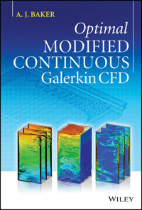
Covers the theory and applications of using weak form theory in incompressible fluid-thermal sciences

Giving you a solid foundation on the Galerkin finite-element method (FEM), this book promotes the use of optimal modified continuous Galerkin weak form theory to generate discrete approximate solutions to incompressible-thermal Navier-Stokes equations. The book covers the topic comprehensively by introducing formulations, theory and implementation of FEM and various flow formulations.

The author first introduces concepts, terminology and methodology related to the topic before covering topics including aerodynamics; the Navier-Stokes Equations; vector field theory implementations and large eddy simulation formulations.

• Introduces and addresses many different flow models (Navier-Stokes, full-potential, potential, compressible/incompressible) from a unified perspective
• Focuses on Galerkin methods for CFD beneficial for engineering graduate students and engineering professionals
• Accompanied by a website with sample applications of the algorithms and example problems and solutions

This approach is useful for graduate students in various engineering fields and as well as professional engineers.

Leseprobe

List of Tables

Table 3.1

Table 3.2

Table 4.1

Table 4.2

Table 4.3

Table 5.1

Table 5.2

Table 6.1

Table 7.1

Table 7.2

Table 8.1

Table 9.1

List of Illustrations

Figure 1.1

Figure 2.1

Figure 2.2

Figure 2.3

Figure 2.4

Figure 2.5

Figure 2.6

Figure 2.7

Figure 2.8

Figure 2.9

Figure 3.1

Figure 3.2

Figure 3.3

Figure 3.4

Figure 3.5

Figure 3.6

Figure 3.7

Figure 3.8

Figure 3.9

Figure 3.10

Figure 3.11

Figure 3.12

Figure 3.13

Figure 3.14

Figure 4.1

Figure 4.2

Figure 4.3

Figure 4.4

Figure 4.5

Figure 4.6

Figure 4.7

Figure 4.8

Figure 4.9

Figure 4.10

Figure 4.11

Figure 4.12

Figure 4.13

Figure 4.14

Figure 4.15

Figure 4.16

Figure 4.17

Figure 4.18

Figure 5.1

Figure 5.2

Figure 5.3

Figure 5.4

Figure 5.5

Figure 5.6

Figure 5.7

Figure 5.8

Figure 5.9

Figure 5.10

Figure 5.11

Figure 5.12

Figure 5.13

Figure 5.14

Figure 5.15

Figure 5.16

Figure 5.17

Figure 6.1

Figure 6.2

Figure 6.3

Figure 6.4

Figure 6.5

Figure 6.6

Figure 6.7

Figure 6.8

Figure 6.9

Figure 6.10

Figure 6.11

Figure 6.12

Figure 6.13

Figure 6.14

Figure 6.15

Figure 6.16

Figure 6.17

Figure 6.18

Figure 7.1

Figure 7.2

Figure 7.3

Figure 7.4

Figure 7.5

Figure 7.6

Figure 7.7

Figure 7.8

Figure 7.9

Figure 7.10

Figure 7.11

Figure 7.12

Figure 7.13

Figure 7.14

Figure 7.15

Figure 7.16

Figure 7.17

Figure 7.18

Figure 7.19

Figure 7.20

Figure 7.21

Figure 7.22

Figure 7.23

Figure 7.24

Figure 7.25

Figure 7.26

Figure 7.27

Figure 7.28

Figure 7.29

Figure 7.30

Figure 7.31

Figure 7.32

Figure 7.33

Figure 7.34

Figure 7.35

Figure 7.36

Figure 7.37

Figure 7.38

Figure 7.39

Figure 7.40

Figure 7.41

Figure 7.42

Figure 7.43

Figure 7.44

Figure 7.45

Figure 7.46

Figure 7.47

Figure 7.48

Figure 8.1

Figure 8.2

Figure 8.3

Figure 8.4

Figure 8.5

Figure 8.6

Figure 8.7

Figure 8.8

Figure 8.9

Figure 8.10

Figure 8.11

Figure 8.12

Figure 8.13

Figure 8.14

Figure 8.15

Figure 8.16

Figure 8.17

Figure 8.18

Figure 8.19

Figure 8.20

Figure 8.21

Figure 8.22

Figure 9.1

Figure 9.2

Figure 9.3

Figure 9.4

Figure 9.5

Figure 9.6

Figure 9.7

Figure 9.8

Figure 9.9

Figure 9.10

Figure 9.11

Figure 9.12

Figure 9.13

Figure 9.14

Figure 9.15

Figure 9.16

Figure 9.17

Figure 9.18

Figure 9.19

Figure 9.20

Figure 9.21

Figure 9.22

Figure 9.23

Figure 9.24

Figure 9.25

Figure 9.26

Figure 9.27

Figure 9.28

Figure 9.29

Figure 9.30

Figure 9.31

Figure 9.32

Figure 9.33

Figure 9.34

Figure 9.35

Figure 9.36

Figure 9.37

Figure 9.38

Figure 9.39

Figure 9.40

Figure 9.41

Figure 9.42

Figure 9.43

Figure 9.44

Figure 9.45

Figure 9.46

Figure 9.47

Figure 9.48

Figure 9.49

Figure 9.50

Guide

Cover

Table of Contents

Preface

Chapter 1

Pages

iii

iv

v

xiii

xiv

xv

xvi

xvii

xix

xx

xxi

xxii

xxiii

xxiv

1

2

3

4

5

6

7

8

9

10

11

12

13

14

15

16

17

18

18

19

20

21

22

23

24

25

26

27

28

29

30

31

32

33

34

35

36

37

38

39

40

41

42

43

44

45

46

47

48

49

50

51

52

53

54

55

56

57

58

59

60

61

62

63

64

65

66

67

68

69

70

71

72

73

74

75

76

77

78

79

80

81

82

83

84

85

86

87

88

89

90

91

92

93

94

95

96

97

98

99

100

101

102

103

104

105

106

107

108

109

110

111

112

113

114

115

116

117

118

119

120

121

122

123

124

125

126

127

128

129

130

131

132

133

134

135

136

137

138

139

140

141

142

143

144

145

146

147

148

149

150

151

152

153

154

155

156

157

158

159

160

161

162

163

164

165

166

167

168

169

170

171

172

173

174

175

176

177

178

179

180

181

182

183

184

185

186

187

188

189

190

191

192

193

194

195

196

197

198

199

200

201

202

203

204

205

206

207

208

209

210

211

212

213

214

215

216

217

218

219

220

221

222

223

224

225

226

227

228

229

230

231

232

233

234

235

236

237

238

239

240

241

242

243

244

245

246

247

248

249

250

251

252

253

254

255

256

257

258

259

260

261

262

263

264

265

266

267

268

269

270

271

272

273

274

275

276

277

278

279

280

281

282

283

284

285

286

287

288

289

290

291

292

293

294

295

296

297

298

299

300

301

302

303

304

305

306

307

308

309

310

311

312

313

314

315

316

317

318

319

320

321

322

323

324

325

326

327

328

329

330

331

332

333

334

335

336

337

338

339

340

341

342

343

344

345

346

347

348

349

350

351

352

353

354

355

356

357

358

359

360

361

362

363

364

365

366

367

368

369

370

371

372

373

374

375

376

377

378

379

380

381

382

383

384

385

386

387

388

389

390

391

392

393

394

395

396

397

398

399

400

401

402

403

404

405

406

407

408

409

410

411

412

413

414

415

416

417

418

419

420

421

422

423

424

425

426

427

428

429

430

431

432

433

434

435

436

437

438

439

440

441

442

443

444

445

446

447

448

449

450

451

452

453

454

455

456

457

458

459

460

461

462

463

464

465

466

467

468

469

470

471

472

473

474

476

477

478

479

480

481

482

483

485

486

487

488

489

490

491

492

493

494

495

496

497

498

499

500

501

502

503

504

505

506

507

508

509

510

511

512

513

514

515

516

517

518

519

520

521

522

523

524

525

526

527

528

529

530

531

532

533

534

535

536

537

538

539

540

541

542

543

544

545

546

547

548

549

550

Optimal Modified Continuous Galerkin CFD

A. J. Baker

Professor EmeritusThe University of Tennessee, USA

This edition first published 2014

© 2014 John Wiley & Sons Ltd

Registered office

John Wiley & Sons Ltd, The Atrium, Southern Gate, Chichester, West Sussex, PO19 8SQ, United Kingdom

For details of our global editorial offices, for customer services and for information about how to apply for permission to reuse the copyright material in this book please see our website at www.wiley.com.

The right of the author to be identified as the author of this work has been asserted in accordance with the Copyright, Designs and Patents Act 1988.

All rights reserved. No part of this publication may be reproduced, stored in a retrieval system, or transmitted, in any form or by any means, electronic, mechanical, photocopying, recording or otherwise, except as permitted by the UK Copyright, Designs and Patents Act 1988, without the prior permission of the publisher.

Wiley also publishes its books in a variety of electronic formats. Some content that appears in print may not be available in electronic books.

Designations used by companies to distinguish their products are often claimed as trademarks. All brand names and product names used in this book are trade names, service marks, trademarks or registered trademarks of their respective owners. The publisher is not associated with any product or vendor mentioned in this book.

Limit of Liability/Disclaimer of Warranty: While the publisher and author have used their best efforts in preparing this book, they make no representations or warranties with respect to the accuracy or completeness of the contents of this book and specifically disclaim any implied warranties of merchantability or fitness for a particular purpose. It is sold on the understanding that the publisher is not engaged in rendering professional services and neither the publisher nor the author shall be liable for damages arising herefrom. If professional advice or other expert assistance is required, the services of a competent professional should be sought.

Library of Congress Cataloging-in-Publication Data

Baker, A. J., 1936–

Optimal modified continuous Galerkin CFD / A. J. Baker.

pages cm

Includes bibliographical references and index.

ISBN 978-1-119-94049-4 (hardback)

1. Fluid mechanics. 2. Finite element method. 3. Galerkin methods. I. Title.

TA357.B273 2014

518′.63—dc23

2013049543

A catalogue record for this book is available from the British Library.

ISBN 9781119940494

Dedication

Yogi Berra is quoted,

“If you come to a fork in the road take it.”

With Mary Ellen's agreement,

following this guidance

I found myself at the

dawning of weak form CFD

Preface

Fluid dynamics, with heat/mass transport, is the engineering sciences discipline wherein explicit nonlinearity fundamentally challenges analytical theorization. Prior to digital computer emergence, hence computational fluid dynamics (CFD), the subject of this text, the regularly revised monograph Boundary Layer Theory, Schlichting (1951, 1955, 1960, 1968, 1979) archived Navier–Stokes (NS) knowledge analytical progress. Updates focused on advances in characterizing turbulence, the continuum phenomenon permeating genuine fluid dynamics. The classic companion for NS simplified to the hyperbolic form, which omits viscous-turbulent phenomena while admitting non-smooth solutions, is Courant et al. (1928).

The analytical subject of CFD is rigorously addressed herein via what has matured as optimal modified continuous Galerkin weak form theory. The predecessor burst onto the CFD scene in the early 1970s disguised as the weighted-residuals finite element (FE) alternative to finite difference (FD) CFD. Weighted-residuals obvious connections to variational calculus prompted mathematical formalization, whence emerged continuum weak form theory. It is this theory, discretely implemented, herein validated precisely pertinent to nonlinear(!) NS, and time averaged and space filtered alternatives, elliptic boundary value (EBV) partial differential equation (PDE) systems.

Pioneering weighted-residuals CFD solutions proved reasonable compared with expectation and comparative data. Reasonable was soon replaced with rigor, first via laminar and turbulent boundary layer (BL) a posteriori data which validated linear weak form theory-predicted optimal performance within the discrete peer group, Soliman and Baker (1981a,b). Thus matured NS weak form theorization in continuum form, whence discrete implementation became a post-theory decision. As thoroughly detailed herein, the FE trial space basis choice is validated optimal in classic and weak form theory-identified norms. Further, this decision uniquely retains calculus and vector field theory supporting computable form generation precision.

Text focus is derivation and thorough quantitative assessment of optimal modified continuous Galerkin CFD algorithms for incompressible laminar-thermal NS plus the manipulations for turbulent and transitional flow prediction. Optimality accrues to continuum alteration of classic text NS PDE statements via rigorously derived nonlinear differential terms. Referenced as modified PDE (mPDE) theory, wide ranging a posteriori data quantitatively validate the theory-generated dispersive/anti-dispersive operands annihilate significant order discrete approximation error in space and time, leading to monotone solution prediction without an artificial diffusion operator.

Weak formulations in the computational engineering sciences, especially fluid dynamics, have a storied history of international contributions. Your author's early 1970s participation culminated in leaving the Bell Aerospace principal research scientist position in 1975 to initiate the University of Tennessee (UT) Engineering Science graduate program focusing in weak form CFD. UT CFD Laboratory, formed in 1982, fostered collaboration among aerospace research technical colleagues, graduate students, commercial industry and the UT Joint Institute for Computational Science (JICS), upon its founding in 1993.

As successor to the 1983 text Finite Element Computational Fluid Mechanics, this book organizes the ensuing three decades of research generating theory advances leading to rigorous, efficient, optimal performance Galerkin CFD algorithm identification. The book is organized into 10 chapters, Chapter 1 introducing the subject content in perspective with an historical overview. Since postgraduate level mathematics are involved, Chapter 2 provides pertinent subject content overview to assist the reader in gaining the appropriate analytical dexterity. Chapter 3 and 4 document weak interaction aerodynamics, the union of potential flow NS with Reynolds-ordered BL theory, laminar and time averaged turbulent, with extension to parabolic NS (PNS) with PNS-ordered full Reynolds stress tensor algebraic closure. Linearity of the potential EBV enables a thoroughly formal derivation of continuum weak form theory via bilinear forms. Content concludes with optimal algorithm identification with an isentropic (weak) shock validation. An Appendix extends the theory to a Reynolds-ordered turbulent hypersonic shock layer aerothermodynamics formulation (PRaNS).

Chapter 5 presents a thorough derivation of mPDE theory generating the weak form optimal performance modified Galerkin algorithm, in time for linear through cubic trial space bases, and in space for optimally efficient linear basis. Theory assertion of optimality within the discrete peer group is quantitatively verified/validated. Chapter 6 validates the algorithm for laminar-thermal NS PDE system arranged to well-posed using vector field theory. Chapter 7 complements content with algorithm validation for the classic state variable laminar-thermal NS system, rendered well-posed via pressure projection theory with a genuine pressure weak formulation pertinent to multiply-connected domains. Content derives/validates a Galerkin theory for radiosity theory replacing Stephan–Boltzmann, also an ALE algorithm for thermo-solid-fluid interaction with melting and solidification.

Chapter 8 directly extends Chapter 7 content to time averaged NS (RaNS) for single Reynolds stress tensor closure models, standard deviatoric and full Reynolds stress model (RSM). Chapter 9 addresses space filtered NS (LES) with focus the Reynolds stress quadruple formally generated by filtering. Manipulations rendering RaNS and LES EBV statements identical lead to closure summary via subgrid stress (SGS) tensor modeling. The alternative completely model-free closure (arLES) for the full tensor quadruple is derived via union of rational LES (RLES) and mPDE theories. Thus is generated an O(1, δ2, δ3) member state variable for gaussian filter uniform measure δ a priori defining unresolved scale threshold. Extended to bounded domains, arLES EBV system including boundary convolution error (BCE) integrals is rendered well-posed via derivation of non-homogeneous Dirichlet BCs for the complete state variable. The arLES theory is validated applicable ∀ Re, generates δ-ordered resolved-unresolved scale diagnostic a posteriori data, and confirms model-free prediction of laminar-turbulent wall attached resolved scale velocity transition.

Chapter 10 collates text content under the US National Academy of Sciences (NAS) large scale computing identification “Verification, Validation, Uncertainly Quantification” (VVUQ). Observed in context is replacement of legacy CFD algorithm numerical diffusion formulations with proven mPDE operand superior performance. More fundamental is the ∀Re model-free arLES theory specific responses to NAS-cited requirements:

error

quantification

a posteriori

error

estimation

error

bounding

spectral content accuracy

extremization

phase selective

dispersion

error annihilation

monotone

solution generation

error

extremization

optimal mesh quantification

mesh resolution

inadequacy

measure

efficient optimal

radiosity

theory with error

bound

which in summary address in completeness VVUQ.

Your author must acknowledge that the content of this text is the result of collaborative activities conducted over three decades under the umbrella of the UT CFD Lab, especially that resulting from PhD research. Content herein is originally published in the dissertations of Doctors Soliman (1978), Kim (1987), Noronha (1988), Iannelli (1991), Freels (1992), Williams (1993), Roy (1994), Wong (1995), Zhang (1995), Chaffin (1997), Kolesnikov (2000), Barton (2000), Chambers (2000), Grubert (2006), Sahu (2006) and Sekachev (2013), the last one completed in the third year of my retirement. During 1977–2006 the UT CFD Lab research code enabling weak form theorization transition to a posteriori data generation was the brainchild of Mr Joe Orzechowski, the maturation of a CFD technical association initiated in 1971 at Bell Aerospace. The unsteady fully 3-D a posteriori data validating arLES theory was generated using the open source, massively parallel PICMSS (Parallel Interoperable Computational Mechanics Systems Simulator) platform, a CFD Lab collaborative development led by Dr Kwai Wong, Research Scientist at JICS.

Teams get the job done – this text is proof positive.

A. J. BakerKnoxville, TNNovember 2013

About the Author

A. J. Baker, PhD, PE, left commercial aerospace research to join The University of Tennessee College of Engineering in 1975, with the goal to initiate a graduate academic research program in the exciting new field of CFD. Now Professor Emeritus and Director Emeritus of the University's CFD Laboratory (http://cfdlab.utk.edu), his professional career started in 1958 as a mechanical engineer with Union Carbide Corp. He departed after five years to enter graduate school full time to “learn what a computer was and could do.” A summer 1967 digital analyst internship with Bell Aerospace Company led to the 1968 technical report “A Numerical Solution Technique for a Class of Two-Dimensional Problems in Fluid Dynamics Formulated via Discrete Elements,” a pioneering expose in the fledgling field of finite-element (FE) CFD. Finishing his (plasma physics topic) dissertation in 1970, he joined Bell Aerospace as Principal Research Scientist to pursue fulltime FE CFD theorization. NASA Langley Research Center stints led to summer appointments at their Institute for Computer Applications in Science and Engineering (ICASE), which in turn led to a 1974–1975 visiting professorship at Old Dominion University. He transitioned directly to UT and in the process founded Computational Mechanics Consultants, Inc., with two Bell Aerospace colleagues, with the mission to convert FE CFD theory academic research progress into computing practice.

Notations

a

expansion coefficient; speed of sound; characteristics coefficient

A

plane area; 1-D FE matrix prefix; coefficient

AD

approximate deconvolution

ADBC

approximate deconvolution boundary condition algorithm

AF

approximate factorization algorithm

ALE

arbitrary-lagrangian-eulerian algorithm

[A]

factored global matrix, RLES theory auxiliary problem matrix operator

ar

LES

essentially analytic LES closure theory

b

coefficient; boundary condition subscript

{b}

global data matrix

B

2-D FE matrix prefix

B(•)

bilinear form

B

body force

BC

boundary condition

BCE

boundary commutation error integral

BHE

borehole heat exchanger

BiSec

bisected borehole heat exchanger

BL