Business Risk and Simulation Modelling in Practice E-Book

Michael Rees

• Herausgeber: John Wiley & Sons
• Kategorie: Fachliteratur
• Serie: Wiley Finance Series
• Sprache: Englisch

Seitenzahl: 794

Veröffentlichungsjahr: 2015

Beschreibung

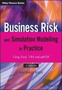
The complete guide to the principles and practice of risk quantification for business applications. The assessment and quantification of risk provide an indispensable part of robust decision-making; to be effective, many professionals need a firm grasp of both the fundamental concepts and of the tools of the trade. Business Risk and Simulation Modelling in Practice is a comprehensive, in-depth, and practical guide that aims to help business risk managers, modelling analysts and general management to understand, conduct and use quantitative risk assessment and uncertainty modelling in their own situations. Key content areas include: * Detailed descriptions of risk assessment processes, their objectives and uses, possible approaches to risk quantification, and their associated decision-benefits and organisational challenges. * Principles and techniques in the design of risk models, including the similarities and differences with traditional financial models, and the enhancements that risk modelling can provide. * In depth coverage of the principles and concepts in simulation methods, the statistical measurement of risk, the use and selection of probability distributions, the creation of dependency relationships, the alignment of risk modelling activities with general risk assessment processes, and a range of Excel modelling techniques. * The implementation of simulation techniques using both Excel/VBA macros and the @RISK Excel add-in. Each platform may be appropriate depending on the context, whereas the core modelling concepts and risk assessment contexts are largely the same in each case. Some additional features and key benefits of using @RISK are also covered. Business Risk and Simulation Modelling in Practice reflects the author's many years in training and consultancy in these areas. It provides clear and complete guidance, enhanced with an expert perspective. It uses approximately one hundred practical and real-life models to demonstrate all key concepts and techniques; these are accessible on the companion website.

Leseprobe

For other titles in the Wiley Finance series please see www.wiley.com/finance

Business Risk and Simulation Modelling in Practice

Using Excel, VBA and @RISK

MICHAEL REES

This edition first published 2015 © 2015 John Wiley & Sons Ltd

Registered officeJohn Wiley & Sons Ltd, The Atrium, Southern Gate, Chichester, West Sussex, PO19 8SQ, United Kingdom

For details of our global editorial offices, for customer services and for information about how to apply for permission to reuse the copyright material in this book please visit our website at www.wiley.com.

All rights reserved. No part of this publication may be reproduced, stored in a retrieval system, or transmitted, in any form or by any means, electronic, mechanical, photocopying, recording or otherwise, except as permitted by the UK Copyright, Designs and Patents Act 1988, without the prior permission of the publisher.

Wiley publishes in a variety of print and electronic formats and by print-on-demand. Some material included with standard print versions of this book may not be included in e-books or in print-on-demand. If this book refers to media such as a CD or DVD that is not included in the version you purchased, you may download this material at http://booksupport.wiley.com. For more information about Wiley products, visit www.wiley.com.

Designations used by companies to distinguish their products are often claimed as trademarks. All brand names and product names used in this book are trade names, service marks, trademarks or registered trademarks of their respective owners. The publisher is not associated with any product or vendor mentioned in this book.

Limit of Liability/Disclaimer of Warranty: While the publisher and author have used their best efforts in preparing this book, they make no representations or warranties with respect to the accuracy or completeness of the contents of this book and specifically disclaim any implied warranties of merchantability or fitness for a particular purpose. It is sold on the understanding that the publisher is not engaged in rendering professional services and neither the publisher nor the author shall be liable for damages arising herefrom. If professional advice or other expert assistance is required, the services of a competent professional should be sought.

Library of Congress Cataloging-in-Publication Data

Rees, Michael, 1964–    Business risk and simulation modelling in practice : using Excel, VBA and @RISK / Michael Rees.       pages cm    Includes index.    ISBN 978-1-118-90405-3 (cloth)  1. Risk management--Computer simulation.   2. Risk management--Data processing.   3. Microsoft Excel (Computer file)   I. Title.    HD61.R44 2015    658.15′50285554--dc23

2015019955

A catalogue record for this book is available from the British Library.

ISBN 978-1-118-90405-3 (hbk) ISBN 978-1-118-90403-9 (ebk) ISBN 978-1-118-90404-6 (ebk) ISBN 978-1-118-90402-2 (ebk)

Cover Design: Wiley Cover Image: ©iStock.com/Mordolff

To my wife and children

CONTENTS

Preface

About the Author

About the Website

PART I An Introduction to Risk Assessment – Its Uses, Processes, Approaches, Benefits and Challenges

CHAPTER 1 The Context and Uses of Risk Assessment

1.1 Risk Assessment Examples

1.2 General Challenges in Decision-Making Processes

1.3 Key Drivers of the Need for Formalised Risk Assessment in Business Contexts

1.4 The Objectives and Uses of General Risk Assessment

CHAPTER 2 Key Stages of the General Risk Assessment Process

2.1 Overview of the Process Stages

2.2 Process Iterations

2.3 Risk Identification

2.4 Risk Mapping

2.5 Risk Prioritisation and Its Potential Criteria

2.6 Risk Response: Mitigation and Exploitation

2.7 Project Management and Monitoring

CHAPTER 3 Approaches to Risk Assessment and Quantification

3.1 Informal or Intuitive Approaches

3.2 Risk Registers without Aggregation

3.3 Risk Register with Aggregation (Quantitative)

3.4 Full Risk Modelling

CHAPTER 4 Full Integrated Risk Modelling: Decision-Support Benefits

4.1 Key Characteristics of Full Models

4.2 Overview of the Benefits of Full Risk Modelling

4.3 Creating More Accurate and Realistic Models

4.4 Using the Range of Possible Outcomes to Enhance Decision-Making

4.5 Supporting Transparent Assumptions and Reducing Biases

4.6 Facilitating Group Work and Communication

CHAPTER 5 Organisational Challenges Relating to Risk Modelling

5.1 “We Are Doing It Already”

5.2 “We Already Tried It, and It Showed Unrealistic Results”

5.3 “The Models Will Not Be Useful!”

5.4 Working Effectively with Enhanced Processes and Procedures

5.5 Management Processes, Culture and Change Management

PART II The Design of Risk Models – Principles, Processes and Methodology

CHAPTER 6 Principles of Simulation Methods

6.1 Core Aspects of Simulation: A Descriptive Example

6.2 Simulation as a Risk Modelling Tool

6.3 Sensitivity and Scenario Analysis: Relationship to Simulation

6.4 Optimisation Analysis and Modelling: Relationship to Simulation

6.5 Analytic and Other Numerical Methods

6.6 The Applicability of Simulation Methods

CHAPTER 7 Core Principles of Risk Model Design

7.1 Model Planning and Communication

7.2 Sensitivity-Driven Thinking as a Model Design Tool

7.3 Risk Mapping and Process Alignment

7.4 General Dependency Relationships

7.5 Working with Existing Models

CHAPTER 8 Measuring Risk using Statistics of Distributions

8.1 Defining Risk More Precisely

8.2 Random Processes and Their Visual Representation

8.3 Percentiles

8.4 Measures of the Central Point

8.5 Measures of Range

8.6 Skewness and Non-Symmetry

8.7 Other Measures of Risk

8.8 Measuring Dependencies

CHAPTER 9 The Selection of Distributions for Use in Risk Models

9.1 Descriptions of Individual Distributions

9.2 A Framework for Distribution Selection and Use

9.3 Approximation of Distributions with Each Other

CHAPTER 10 Creating Samples from Distributions

10.1 Readily Available Inverse Functions

10.2 Functions Requiring Lookup and Search Methods

10.3 Comparing Calculated Samples with Those in @RISK

10.4 Creating User-Defined Inverse Functions

10.5 Other Generalisations

CHAPTER 11 Modelling Dependencies between Sources of Risk

11.1 Parameter Dependency and Partial Causality

11.2 Dependencies between Sampling Processes

11.3 Dependencies within Time Series

PART III Getting Started with Simulation in Practice

CHAPTER 12 Using Excel/VBA for Simulation Modelling

12.1 Description of Example Model and Uncertainty Ranges

12.2 Creating and Running a Simulation: Core Steps

12.3 Basic Results Analysis

12.4 Other Simple Features

12.5 Generalising the Core Capabilities

12.6 Optimising Model Structure and Layout

12.7 Bringing it All Together: Examples Using the Simulation Template

12.8 Further Possible uses of VBA

CHAPTER 13 Using @RISK for Simulation Modelling

13.1 Description of Example Model and Uncertainty Ranges

13.2 Creating and Running a Simulation: Core Steps and Basic Icons

13.3 Simulation Control: An Introduction

13.4 Further Core Features

13.5 Working with Macros and the @RISK Macro Language

13.6 Additional In-Built Applications and Features: An Introduction

13.7 Benefits of @RISK over Excel/VBA Approaches: A Brief Summary

Index

EULA

List of Tables

Chapter 9

Table 9.1

List of Illustrations

Chapter 1

Figure 1.1

Number of Successful Projects out of 100, Each with Probability of Success Equal to 30%

Figure 1.2

Number of Successful Projects out of 10, Each with Probability of Success Equal to 60%

Figure 1.3

Number of Projects Required to have Six Successes, where Each has a 60% Probability of Success

Chapter 3

Figure 3.1

Example of a Generic Qualitative Risk Register

Figure 3.2

Example of a Generic Quantitative Risk Register Without Aggregation

Figure 3.3

Example of a Generic Quantitative Risk Register with Aggregation of Static Values

Figure 3.4

Example of a Generic Quantitative Risk Register with Aggregation of Uncertain Values

Figure 3.5

Distribution of Outcome for Quantitative Risk Register with Aggregation of Uncertain Values

Chapter 4

Figure 4.1

Original Model of Price Development

Figure 4.2

Revised Plan for Price Development Assuming Successful Upgrade at Each Step

Figure 4.3

Revised Plan for Price Development Assuming Uncertainty of the Success of the Upgrade at Each Step

Figure 4.4

Translation of Wind Speed into Power Output

Figure 4.5

Assumed Distribution of Wind Speed

Figure 4.6

Simulated Distribution of Power Output

Figure 4.7

Ten-year Forecast of Total Expenditure for Each Fuel Type, Using Static Growth Assumptions

Figure 4.8

Ten-year Forecast of Total Expenditure for each Fuel Type, Using Static Growth Assumptions and Including a Switching Option

Figure 4.9

Ten-year Forecast of Total Expenditure for each Fuel Type, Using Uncertain Growth Assumptions and Including A Switching Option

Figure 4.10

Model of Project Duration (Base Case View)

Figure 4.11

Model of Project Cost (Base Case View)

Figure 4.12

Simulated Distribution of Project Duration

Figure 4.13

Simulated Distribution of Project Cost

Figure 4.14

Simulated Distribution of Project Duration Against Cost

Figure 4.15

Simulated Total Travel Time for 10 Days and 100 Days

Figure 4.16

Cost Budget with Each Base Case Value Equal to the P40 of its Distribution

Figure 4.17

Assumed Cost Distribution for Each Item

Figure 4.18

Simulated Distribution of Total Cost

Figure 4.19

Mapping of Base Case Percentiles to Output Percentiles for 10 Symmetric Inputs

Figure 4.20

Mapping of Base Case Percentiles to Output Percentiles for 10 Symmetric and Non-symmetric Inputs

Figure 4.21

Mapping of Base Case Percentiles to Output Percentiles for Various Numbers of Symmetric Inputs

Chapter 6

Figure 6.1

Number of Possible Combinations of Values for Various Numbers of Inputs, where Each Input can Take One of Three Values

Figure 6.2

Number of Combinations Involving Inputs Taking a Particular Number of High or Low Values

Figure 6.3

Percentages of Combinations Involving Inputs Taking a Particular Number of High or Low Values

Figure 6.4

Simulated Distribution of Output Values for Uniform Continuous Inputs

Figure 6.5

Generic Business Plan with Static Inputs

Figure 6.6

Sensitivity Analysis of NPV to Growth Rate in Volume

Figure 6.7

Business Plan with Flexible Start Date for Capital Expenditure and Production Volume

Figure 6.8

Sensitivity Analysis of NPV to Start Dates

Figure 6.9

Sensitivity Analysis of NPV to Start Dates and Growth Rate in Volume

Figure 6.10

Business Plan Model Adapted to Include Input Scenarios

Figure 6.11

Sensitivity Analysis of NPV to Scenario

Figure 6.12

Finding the Required Growth Rate to Achieve a Target NPV

Figure 6.13

Relationship Between Sensitivities, Uncertainty and Optimisation

Figure 6.14

Project Portfolio with Mapping from Generic Time Axis to Specific Dates

Figure 6.15

Delayed Launch Dates to Some Projects may Create an Acceptable or Optimal Solution

Figure 6.16

The Solver Dialog Box

Figure 6.17

Categories of Optimisation Situations

Figure 6.18

Simple Example of a Decision Structure

Figure 6.19

Sequential Decisions Presented as a Single Full Decision Set

Figure 6.20

Simple Example of Decision Tree with Future Uncertainty

Figure 6.21

Decision Tree with Decisions Taken Following an Uncertain Outcome

Figure 6.22

Excel Backward Calculation Path to Replicate Decision Tree Logic

Chapter 7

Figure 7.1

Use of Model Switch to Use Either a Base or a Risk Case Within the Model

Figure 7.2

Calculation of NPV for a Simple Project

Figure 7.3

NPV for Three Decision Options

Figure 7.4

Tornado Chart for Decision Options

Figure 7.5

Tornado Chart for Uncertainties Within a Decision Option

Figure 7.6

Simple Resource Plan

Figure 7.7

Resource Plan with First Approach to Calculations

Figure 7.8

Resource Plan with Second Approach to Calculations

Figure 7.9

Resource Plan with Uncertainty Ranges

Figure 7.10

Distribution of Total Resource Requirements

Figure 7.11

Various Approaches to Implementing Time Shifting in Excel

Figure 7.12

Calculations of Aggregate Delay As an Uncertain Amount

Figure 7.13

Cost Budget with Independent Items

Figure 7.14

Cost Budget with a Common Driver

Figure 7.15

Scenarios for Price Development

Figure 7.16

Price Development in Each Scenario, Using Sensitivity Analysis

Figure 7.17

Detailed Cost Budget Without Categories

Figure 7.18

Detailed Cost Budget with two Types of Category

Figure 7.19

Summary of Cost Budget by Each Type of Category

Figure 7.20

Detailed Cost Budget with Risk Categories

Figure 7.21

Summary of Cost Budget by Risk Category

Figure 7.22

Sensitivity Analysis of Cost Budget by Risk Category

Figure 7.23

Sensitivity Analysis of Cost Budget for Two Risk Categories

Figure 7.24

Uncertainty Model of Cost Budget by Risk Category

Figure 7.25

Simulated Distribution of Total Costs, Comparing Individual Independent Items Versus the Use of Risk Categories

Figure 7.26

Simulated Distribution of Costs by Presentation Category

Figure 7.27

Various Possible Implementations of Fade Formulae

Figure 7.28

Approaches to Aggregating the Effect of Improvement Initiatives: Addition of Static Values

Figure 7.29

Approaches to Aggregating the Effect of Improvement Initiatives: Multiplication of Static Values

Figure 7.30

Approaches to Aggregating the Effect of Improvement Initiatives: Weighting Factors of Static Values

Figure 7.31

Approaches to Aggregating the Effect of Improvement Initiatives: Uncertainty Ranges Around the Selected Static Approach (Excel)

Figure 7.32

Approaches to Aggregating the Effect of Improvement Initiatives: Uncertainty Ranges Around the Selected Static Approach (@RISK)

Figure 7.33

Working with Only the Maximum Impact Within a Category

Figure 7.34

Controlling a Model Switch with a VBA Macro

Figure 7.35

Clearing Filters with a VBA Macro

Figure 7.36

Running Sensitivities with a VBA Macro

Chapter 8

Figure 8.1

Example of a Probability Density Curve for a Continuous Process

Figure 8.2

Example of a Cumulative Curve for a Continuous Process

Figure 8.3

Example of a Descending Cumulative Curve for a Continuous Process

Figure 8.4

Example of Distribution for an Event Risk (Bernoulli or Binomial)

Figure 8.5

Example of a Compound Distribution: Density Curve

Figure 8.6

Example of a Compound Distribution: Cumulative Curve

Figure 8.7

Standard Normal Distribution, Containing Approximately 84% of Occurrences in the Range from Infinity to One Standard Deviation Above the Mean

Figure 8.8

Inversion of the Standard Normal Distribution: Finding the Point Below which Approximately 84% of Outcomes Arise

Figure 8.9

Hypothesised Input Distribution for Cost Example

Figure 8.10

Normal Distribution with Average of 10 and Standard Deviation of 5; Approximately 68% of Outcomes are within the Range that is One Standard Deviation Either Side of the Mean

Figure 8.11

The One Standard Deviation Bands for the Hypothesised Cost Distribution

Figure 8.12

Comparison of Normal Distributions with Various Standard Deviations

Figure 8.13

The One Standard Deviation for the Bernoulli (Binomial) Distribution Contains the Bar with the Larger Probability

Figure 8.14

Example of a Lognormal Distribution

Figure 8.15

A Special Case of a Distribution with Zero Skewness

Figure 8.16

A Special Case of a Positively Skewed Distribution Whose Mean is Less than its Mode

Figure 8.17

A Special Case of a Positively Skewed Distribution with Identical Mean, Median and Mode

Figure 8.18

The Kurtosis of a Discrete Process may Decrease as Tail Events Become Less Likely

Figure 8.19

Simple Example of the Calculation of the Semi-Deviation of a Data Set

Figure 8.20

Initial Given Data on Probabilities

Figure 8.21

Completed Data on Probabilities

Figure 8.22

Data on Probabilities that would Apply for Independent Processes

Figure 8.23

Calculation of Pearson and of Rank Correlation

Figure 8.24

A Scatter Plot and its Associated Regression Line

Chapter 9

Figure 9.1

An Example of a Uniform Continuous Distribution

Figure 9.2

An Example of a Bernoulli Distribution

Figure 9.3

Binomial Distribution Calculations in Excel

Figure 9.4

An Example of a Binomial Distribution

Figure 9.5

An Example of a Triangular Distribution

Figure 9.6

Normal Distribution Calculations in Excel

Figure 9.7

An Example of a Binomial Distribution for 100 Events

Figure 9.8

Overlay of a Triangular Approximating Distribution with the Underlying Normal Distribution

Figure 9.9

Calculations to Approximate a Normal with a Triangular Distribution

Figure 9.10

Excel Calculations of a Lognormal Distribution

Figure 9.11

An Example of a Lognormal Distribution

Figure 9.12

Example of Skewness Arising from Multiplicative Processes

Figure 9.13

Further Example of Skewness Arising from Multiplicative Processes

Figure 9.14

Multiplicative Processes Implicit within some Time Series

Figure 9.15

Comparison of Skewness of Input and Reciprocal Distributions

Figure 9.16

An Example of a Beta Distribution

Figure 9.17

A Further Example of a Beta Distribution

Figure 9.18

An Example of PERT and Triangular Distributions

Figure 9.19

Binomial and Poisson Distributions

Figure 9.20

A Low Intensity Poisson Process

Figure 9.21

A High Intensity Poisson Process

Figure 9.22

An Example of a Geometric Distribution

Figure 9.23

An Example of a Negative Binomial Distribution

Figure 9.24

An Example of an Exponential Distribution

Figure 9.25

An Example of a Weibull Distribution

Figure 9.26

Examples of the Gamma Distribution

Figure 9.27

Example Table of Values and Probabilities for the General Discrete Distribution

Figure 9.28

An Example of a Pareto Distribution

Figure 9.29

Simulation of Extreme Values in Order to Compare with Values Derived Using Theory

Figure 9.30

An Example of a Logistic Distribution

Figure 9.31

An Example of a Log-logistic Distribution

Figure 9.32

Comparison of (

t

) Student and Normal Distributions

Figure 9.33

Excel Calculations of Confidence Intervals

Figure 9.34

Comparisons of Various Implementations of the

t

(Student) Distribution

Figure 9.35

Excel Calculations of Weibull Parameters Given Percentile Information

Figure 9.36

Example of a Percentile (Alternate) Parameter Form of the PERT Distribution

Figure 9.37

Comparison of Lognormal and PERT Distributions with the same P10, most Likely and P90 Values

Figure 9.38

Derivation of Weights to Use at the P10, P50 and P90 Values, in Order to Approximate a Normal Distribution with a General Discrete Distribution

Figure 9.39

Using 30-40-30 Weights for Non-normal Distributions will Provide Only an Approximation

Figure 9.40

Using the Exponential Distribution with its P60 Equal to 100

Figure 9.41

Using the Lognormal Distribution with its P60 Equal to 100

Figure 9.42

Using the PERT Distribution with its P60 Equal to 100

Figure 9.43

Comparison of Mean Values for Various Distribution Assumptions

Figure 9.44

Using the Normal Distribution with its P60 Equal to 100

Figure 9.45

Cross-calibration of Probabilities of Occurrence for Time Periods

Figure 9.46

Cross-calibration of Probabilities of Occurrence for Multiple Risks

Chapter 10

Figure 10.1

Examples of Excel Inverse Functions

Figure 10.2

Inverse Functions Calculated Analytically

Figure 10.3

Example of a Lookup Table to Calculate the Inverse

Figure 10.4

Comparison of User-Defined Inverse Functions with Samples from @RISK

Chapter 11

Figure 11.1

An Example of the Use of Conditional Probabilities

Figure 11.2

Conditional Probabilities of Several Events with a Single Risk Driver

Figure 11.3

Conditional Probabilities of Several Events with Several Categories of Risk Driver

Figure 11.4

Portfolios of Projects that Occur in Phases

Figure 11.5

Distribution of Prices for a Reference Product with Uncertainty Ranges within Uncertain Scenarios

Figure 11.6

Distribution of Prices for a Derivative Product with Uncertain Ranges and Base Prices Depending on the Reference Product

Figure 11.7

Distribution of Prices for Several Derivative Products

Figure 11.8

Base Case Values for Rig Cost as a Function of Oil Price

Figure 11.9

Simulated Distribution of Rig Cost and Scatter Plot of Rig Cost Against Oil Price

Figure 11.10

Uncertainty Model for Market Share and Number of Competitors

Figure 11.11

Time Development of Ranges for Market Share

Figure 11.12

Time Development of Distribution of Market Share

Figure 11.13

Example of Resampling Method

Figure 11.14

Declining Correlations as the Independent Range for a Semi-Dependent Variable Increases

Figure 11.15

Cross-Correlations Between Simulated Product Prices

Figure 11.16

Comparison of Effect of Parameter Changes on Samples Drawn for Correlated Variables

Figure 11.17

Example of Percentile Relationships for a Clayton Copula

Figure 11.18

Simulation of Cross-correlations Implied by a Partial Dependency with a Common Risk Driver

Figure 11.19

Model to Simulate Correlated Items Using Correlations Implied by a Common Risk Driver

Figure 11.20

Overlay of Simulated Distributions of Project Totals that Result From Partial Causality and Correlation Relationships

Figure 11.21

Testing the Formula to Generate Two Correlated Samples

Figure 11.22

Calculation of the Cholesky Matrix for Four Variables

Figure 11.23

Creation of the Cholesky Matrix with a User-defined Array Function

Figure 11.24

Creation of Random Samples as Row or Column Vectors with User-defined Functions

Figure 11.25

Example of an Invalid Correlation Matrix

Figure 11.26

Using @RISK's Functionality to Create an Adapted Correlation Matrix

Figure 11.27

Real Options Value of Flexibility when Price Movements are Correlated

Figure 11.28

Various Implementations of the Growth Formulae

Figure 11.29

Comparison of Simulated Means with Original Values for Various Growth Formulae

Figure 11.30

Example of Convexity Effect of Applying Non-linear Formulae to Uncertain Values

Figure 11.31

Example of Moving Average Time Series

Figure 11.32

Example of Autoregressive Time Series

Figure 11.33

Example of GARCH Time Series

Chapter 12

Figure 12.1

Base Cost Model

Figure 12.2

Cost Model with Values Defining the Uncertainty Ranges

Figure 12.3

Cost Model with Uncertainty Distributions

Figure 12.4

The Visual Basic Editor (VBE)

Figure 12.5

Split Screen of Uncertainty Model and VBE with Code Window

Figure 12.6

Basic Simulation Code and First Results

Figure 12.7

Basic Simulation Results and Statistics

Figure 12.8

Basic Simulation Results, Statistics and Graph

Figure 12.9

The VBE Properties Window

Figure 12.10

Use of Separate Worksheet to Reference Output Cells

Figure 12.11

Use of Analysis Sheet that Links Indirectly to Results Sheets

Figure 12.12

Additional Example of Output Analysis: Cross-Correlations of Outputs for a Selected Results Data Set, and Average Values for Each Output for Several Data Sets

Figure 12.13

Adapted Model to Run Multiple Simulations in an Automated Sequence

Figure 12.14

Using the Simulation Template Model: Example 1

Figure 12.15

Using the Simulation Template Model: Example 2

Figure 12.16

Using the Simulation Template Model: Example 3

Figure 12.17

Using the Simulation Template Model: Example 4

Figure 12.18

Using the Simulation Template Model: Example 5

Figure 12.19

Creating a User-defined Array Function to Generate Random Numbers in Rows or Columns

Figure 12.20

Creating a User-defined Array Function to Generate Correlated or Uncorrelated Samples in Rows or Columns

Figure 12.21

Named Range into Which Random Numbers are to be Assigned

Figure 12.22

Completed Range after Assignment of Random Numbers

Figure 12.23

Generation of a Set of Random Numbers Using a Fixed Seed

Figure 12.24

Generation of Sequences of Random Number Sets Using a Fixed Seed

Figure 12.25

Model Used to Compare Speed of Assignment with Use of Functions

Chapter 13

Figure 13.1

Base Cost Model

Figure 13.2

Cost Model with Values Defining the Uncertainty Ranges

Figure 13.3

Core Icons to Build and Run a Simulation Model with @RISK

Figure 13.4

Cost Model with Uncertainty Distributions

Figure 13.5

Defining Properties of an Input Distribution

Figure 13.6

Adding an Output

Figure 13.7

Simulated Distribution of Total Cost

Figure 13.8

Cumulative Ascending Curve for Simulated Total Cost

Figure 13.9

Adapted Model to Run Multiple Simulations in an Automated Sequence

Figure 13.10

Overlaying the Results of Three Simulations

Figure 13.11

Use of @RISK's Insert Function Icon

Figure 13.12

Use of RiskStatistics Functions with Multiple Simulations

Figure 13.13

The Simulation Settings Dialog

Figure 13.14

Adaptation of Random Numbers in Latin Hypercube Sampling

Figure 13.15

Overlay of Excel and @RISK Samples from a Standard Uniform Continuous Distribution

Figure 13.16

Cost Model with Common Driver of Most Likely Values for Each Uncertain Item

Figure 13.17

Scatter Plot of Total Cost Against Unit Labour Cost

Figure 13.18

Tornado Chart of Correlation Coefficients with Smart Sensitivity Analysis Enabled (1000 Iterations)

Figure 13.19

Tornado Chart of Correlation Coefficients with Smart Sensitivity Analysis Enabled (10,000 Iterations)

Figure 13.20

Tornado Chart of Correlation Coefficients with Smart Sensitivity Analysis Disabled

Figure 13.21

Tornado Chart of Regression Coefficients

Figure 13.22

Tornado Chart of Regression Coefficients for Independent Items

Figure 13.23

Tornado Chart of Correlation Coefficients for Independent Items

Figure 13.24

Use of Change in Output Mean Tornado Graphs: Independent Items

Figure 13.25

Use of Change in Output Mean Tornado Graphs: Items with Common Risk Driver

Figure 13.26

Use of Change in Output Mean Tornado Chart for a Model with Variables Acting in Positive and Negative Senses

Figure 13.27

Use of Regression-Mapped Values Tornado Chart for a Model with Variables Acting in Positive and Negative Senses

Figure 13.28

Tornado Chart for a Model with Many Line Items

Figure 13.29

Tornado Chart for a Model with Summary Items Using RiskMakeInput

Figure 13.30

Use of RiskMakeInput as Dummy Cells in a Model

Figure 13.31

Scatter Plot of Total Revenues Against those of North America

Figure 13.32

Tornado Chart of Risks with Separate Occurrence and Impact Distributions

Figure 13.33

Tornado Chart with Occurrence and Impact Aggregated into a Single Risk Factor

Figure 13.34

A Triangular Process as a Compound Distribution

Figure 13.35

A Portfolio of Compound Processes and the Simulated Total Output

Figure 13.36

The Macros Tab of the SimulationSettings Dialog

Figure 13.37

Accessing the XDK Help Menu

Figure 13.38

Model to Calculate π Using the Dartboard Method

Figure 13.39

Summary Results of the Two-dimensional Dartboard Method

Figure 13.40

Model Used to Run the Two-dimensional Dartboard Method

Figure 13.41

Expected Frequency of Hits with the Multi-dimensional Dartboard Method

Figure 13.42

Summary Results of the 10-dimensional Dartboard Method

Figure 13.43

Model to Generate a Set of Correlated Random Numbers

Figure 13.44

Example of Moving Average Time Series Using @RISK

Guide

Cover

Table of Contents

Preface

Pages

xvii

xviii

xix

xx

xxi

xxiii

xxv

1

3

4

5

6

7

8

9

10

11

12

13

14

15

16

17

18

19

20

21

22

23

24

25

26

27

29

30

31

32

33

34

35

36

37

38

39

40

41

42

43

44

45

46

47

48

49

50

51

52

53

54

55

56

57

59

60

61

62

63

64

65

66

67

68

69

70

71

72

73

74

76

77

78

79

80

82

83

84

85

86

87

88

89

90

91

92

93

94

95

96

97

98

99

100

101

102

103

105

107

108

109

110

111

112

113

114

115

116

117

118

119

120

121

122

123

124

125

126

127

128

129

131

132

133

134

135

137

138

139

140

141

143

144

145

146

147

148

149

150

151

152

153

154

155

156

157

158

159

160

161

162

163

164

166

167

168

169

170

171

172

173

174

175

176

177

178

179

181

182

183

184

185

186

187

188

189

190

191

192

193

194

195

196

197

198

199

200

201

202

203

204

205

206

207

208

209

210

212

213

215

216

217

218

219

220

221

222

223

224

225

226

227

228

229

230

231

232

233

234

235

236

237

238

239

240

241

242

243

244

245

246

247

248

250

251

252

253

254

255

256

257

258

259

260

261

262

263

264

265

266

267

268

269

270

271

272

273

274

275

276

277

278

279

280

281

282

283

284

285

286

287

288

289

291

292

293

294

295

296

297

298

299

300

301

302

303

304

305

306

307

308

309

310

311

312

313

314

315

316

317

318

319

320

321

322

323

325

327

328

329

330

331

332

333

334

335

336

337

338

339

340

341

342

343

344

345

346

347

348

349

350

351

352

353

354

355

356

357

358

359

360

361

362

363

364

365

366

367

368

369

370

371

372

373

374

376

377

378

379

380

381

382

383

384

385

386

388

389

390

391

392

395

398

400

403

405

406

407

409

410

411

414

415

416

417

419

420

421

423

425

426

427

428

429

430

431

432

433

434

435

436

437

438

Preface

This book aims to be a practical guide to help business risk managers, modelling analysts and general management to understand, conduct and use quantitative risk assessment and uncertainty modelling in their own situations. It is intended to provide a solid foundation in the most relevant aspects of quantitative modelling and the associated statistical concepts in a way that is accessible, intuitive, pragmatic and applicable to general business and corporate contexts. It also discusses the interfaces between quantitative risk modelling activities and the organisational context within which such activities take place. In particular, it covers links with general risk assessment processes and issues relating to organisational cultures, incentives and change management. Some knowledge of these issues is generally important in order to ensure the success of quantitative risk assessment approaches in practical organisational contexts.